Centres Without Privilege

The Geometry of Market Fragility -Part II: the City of London, the Euro Area, and the Limits of the Backstop

Abstract

The Geometry of Market Fragility - Part I measured how close the US Treasury market sits to a self-amplifying break, and found a structure already past the historical danger marks on every measure. What holds it, for now, is a privilege no other issuer possesses: in a crisis, the United States can create the very asset the crisis demands - US currency. This Part II turns to the centres and sovereigns that cannot. We read three of them through the same multi-lens method — the City of London, the euro area, and, as the benchmark, the United States — and find that the informative comparison is not “how fragile” but where the backstop runs out. Each of the three backstops has a differently-shaped gap, and it is the shape of the gap, not its depth, that determines how each centre would break.

The City of London is the centrepiece. It is the world’s largest centre for foreign exchange, for the clearing of interest-rate derivatives, for offshore dollar funding, for metals, energy and gold, and for marine insurance — yet the currencies it intermediates are, in the main, ones its own central bank cannot issue. On that structure it runs near-critical: an amplification factor of 0.88, against a runaway threshold of 1. Its three large clearing houses are legally separate; a shock placed at any one of them draws on the same collateral pool, so the apparent diversification of London’s clearing does not hold under stress. The Bank of England has built a careful set of facilities and closed the channel that broke in 2022; the residual gap is precise and recognised — non-bank dollar leverage and the cross-clearing-house collateral spiral — and it is where the public data now shows the build-up.

The euro area is the counterpoint. Its backstop is the most powerful of the three in one dimension — the European Central Bank can issue euros without limit — yet the most constrained in another: with no fiscal union, the sovereign backstop must be conditional, and that conditionality binds hardest on the member state into which fragility is now migrating. The euro area’s fragility is not that its central bank is weak. It is that a monetary union without a fiscal union, and with supervision still fragmented across multiple national authorities and settlement systems, cannot backstop unconditionally what a unitary state can.

The result is a map of three centres and three gaps: New York, whose backstop is complete; London, which can issue its own currency but borrows the one it runs on; and the euro area, which can issue the currency it runs on but cannot, by construction, backstop its members without condition. A closing exhibit reads the three as one system: joined by their ten documented cross-centre channels (a replay against the 2011 record adds an eleventh, §5.4), the coupled structure returns an amplification factor above the runaway threshold — each centre alone attenuates a shock, the coupled system amplifies it — while the backstops that hold the whole remain national, and no single one of them spans it.

1. Introduction: the question Part 1 left open

Twice in six years a central bank has had to buy a sovereign’s safe asset to keep it safe — the Federal Reserve in the US Treasury market in March 2020, the Bank of England in the gilt market in October 2022 (Bank of England 2022). Part 1 of this series (Gao 2026a) measured the US case and reached an uncomfortable conclusion: the Treasury complex of 2026 reads, on every structural measure, above the levels seen on the eve of the historical sovereign- and funding-market crises, and what holds it is not a lower fragility but a unique capacity to absorb one. In a dollar crisis the Federal Reserve can create the dollars the crisis is short of. That is privilege, and it is the reason the same structural reading means something different for the United States than for anyone else.

This Part takes the method to the issuers and centres that do not have it. We examine three:

• The United Kingdom, through the City of London — a middle power whose central bank can issue its own currency but whose financial centre runs, in large part, on currencies it cannot.

• The euro area — a monetary union whose central bank can issue the currency the union runs on, but which has no common treasury behind it.

• The United States — carried over from Part 1 as the benchmark of a complete backstop.

The organising idea is backstop reachability: not the size of a fragility, but the question of who can backstop what, and on what condition. Part 1 introduced the containment axis — whether the public sector can catch a forced-selling spiral — as the variable that decides outcomes. Here we make it a property of the network itself. A backstop has a reach: a set of nodes it can stabilise, in a currency it can supply, on terms it can offer. Where the load-bearing nodes of a centre lie outside that reach, the structure has a gap — a place where it can break that no available facility directly covers. The three centres differ less in how amplified they are than in where that gap lies.

The report proceeds from the centrepiece outward. Section 2 sets out the method, the reachability axis, the sensitivity of the readings to their calibration, and the standing of the different claims. Section 3 is the City of London: the 2022 crisis that was caught and the structure that was reformed; the wider complex and why its diversified clearing does not hold under stress; the liquidity it maintains in currencies it cannot issue; and the precise gap in the Bank of England’s toolkit. Section 4 is the euro area: the 2010–12 crisis and its commitment-based containment, the migration of fragility to France today, and why a powerful central bank without a fiscal union has a differently-shaped gap. Section 5 sets the three side by side, and closes with a first structural reading of the three coupled into one system. Section 6 draws out what the no-privilege cases add to the framework and what to watch.

A note on what is and is not new here. The macro frame around much of this — that a core financial cycle drives the periphery, that capital-flow reversals transmit through global banks — is a mature literature, and where we touch it we cite it and build on it (Rey 2013). Our contribution is narrower: the same auditable, reproducible structural method, applied to the actual market infrastructure — the clearing houses, the collateral pools, the funding conduits — and read through the single lens of backstop reachability.

Three tiers of claim run through what follows, and the reader should carry the classification from the start (the full statement is §2.4):

2. Method, sensitivity, and the standing of the claims

2.1 The four structural readings

The method is the one developed and validated in Part 1, and we do not re-derive it here; the formal definitions are in Appendix A, and every network in this report is openable and re-runnable in the accompanying tool. In brief, each financial complex is represented as a directed, weighted network in which an edge from one balance sheet to another carries the fraction of a distress shock that the first transmits to the second when it is forced to act — to sell, to withhold funding, to call collateral. On that representation we read four structural measures:

• The amplification factor is the weighted spectral radius of the network — the single number that summarises how far a shock is multiplied as it circulates around the network’s feedback loops. A value below 1 means a shock dies away; a value approaching 1 means it is amplified without bound; and the steady-state multiplier of an initial shock is one divided by one minus the factor (May 1972). This is the leading measure, because it can be read before any shock arrives.

• The loop-concentration reading asks whether the feedback is carried by one dominant loop — so that a single, well-aimed intervention can break it — or spread across many, so that no single point dominates.

• The keystone reading identifies the node through which the most feedback runs: the natural target for a backstop.

• The cascade simulation propagates a specific shock from a specific origin and reports where the distress comes to rest. We use it to test whether separate-looking parts of a centre are in fact bound together.

2.2 The backstop-reachability axis

To these we add the axis this Part is built on. Backstop reachability classifies, for each centre, what its public sector can stabilise. We resolve it along three concrete dimensions, because that is how the real toolkits are organised:

1. Currency — can the central bank issue the currency in which the load-bearing exposures are denominated? New York: yes (dollars). London: its own currency yes (sterling), but the currency much of its infrastructure runs on, no (dollars). The euro area: yes (euros).

2. Counterparty — does a facility reach the institutions that actually carry the fragility — banks only, or also the non-banks (pension funds, hedge funds, clearing members) that now sit at the centre of these structures?

3. Sovereign capacity and condition — can the backstop be extended unconditionally, as a unitary state backstops its own debt, or only on conditions that may fail precisely when the backstop is most needed?

A centre is well-covered where its keystone and its dominant loops fall inside the reach on all three dimensions. It has a gap where they fall outside. The rest of this report locates those gaps.

2.3 What the readings rest on: sensitivity to calibration error

Each network in this report is calibrated by hand: an edge weight is set by the class of mechanism it represents — a margin or clearing pass-through, a funding withdrawal, a reflexive asset sale — and anchored, where possible, to a documented episode (the per-edge mechanism and source are in Appendix B). A careful reader will ask how much the conclusions depend on those particular numbers. The honest answer is that the precise value of an amplification factor depends on the calibration, and we report it as such; but the qualitative readings — whether a structure sits in the amplifying band, and which node is its keystone — are robust to substantial miscalibration, and we have measured how robust.

The test perturbs every calibrated edge weight in a network by a uniform random factor — plus or minus 15, 20 and 30 per cent — and recomputes the amplification factor and the keystone for each of 2,000 draws at each level, with a fixed random seed so the result is reproducible (Figure 1). For the City of London network, the amplification factor stays inside roughly 0.84 to 0.92 under a 20-per-cent perturbation and does not leave the amplifying band even under a 30-per-cent one; the keystone is the interest-rate-swap clearing house, or in a minority of draws the collateral pool it shares with the others — in every draw, one of the two nodes of the same clearing-and-collateral complex. For the euro-area network the amplification factor stays near 0.96 and the keystone is the Italian sovereign in every draw. The qualitative findings of this report do not turn on the third decimal place of any edge weight.

The reading is therefore the one a central bank would want stated plainly: the precise amplification factor is calibration-dependent and is given as a range; the structural conclusions — amplifying regime, single identifiable keystone — survive a 30-per-cent error applied to every edge at once. One feature is informative rather than reassuring. Under heavy miscalibration the euro-area network’s amplification factor crosses 1 in a meaningful fraction of draws, while London’s does not: a structural statement that the euro area sits closer to the runaway threshold than London — a difference the precise calibration also shows, and one we return to in Section 4.

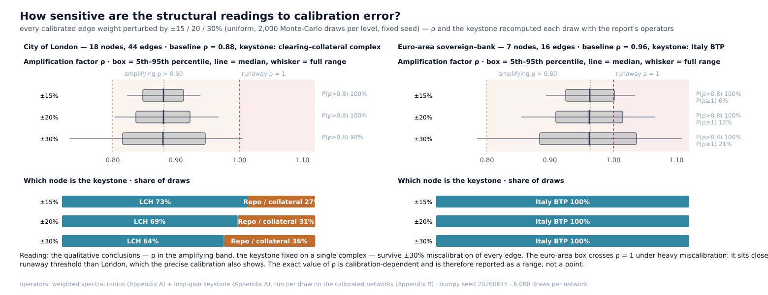
Figure 1 — Sensitivity of the structural readings to calibration error. For the two live Part-2 networks, every calibrated edge weight is perturbed by ±15 / 20 / 30 per cent (uniform, 2,000 Monte-Carlo draws per level, fixed seed); the amplification factor and the keystone are recomputed each draw with the report’s operators. Upper sub-panels: the distribution of the amplification factor (box = 5th–95th percentile, line = median, whisker = full range) against the amplifying band (above 0.80) and the runaway threshold (1.0). Lower sub-panels: the share of draws in which each node is the keystone.

2.4 What the readings do and do not establish

Three classes of claim run through this report, and we label them throughout rather than leave the reader to judge their standing unaided.

• Established. That a weighted feedback network has a runaway threshold at an amplification factor of 1, with a steady-state multiplier of one over one minus the factor, is a result with half a century of standing (May 1972); the reverberating-cascade construction we use to propagate a specific shock is published and widely used (Battiston et al. 2012). Where we rely on these we cite them and do not re-argue them.

• Calibrated and sourced. The networks themselves — which balance sheets, which transmission channels, what weight each carries — are our construction, built from public data, supervisory reports and documented episodes, and labelled edge by edge in Appendix B as either anchored to an episode or estimated by mechanism class. These are arguments from evidence, open to challenge on the evidence; they are not laws.

• Conditional. The forward-looking readings — that a structure is near-critical today, that fragility is migrating, that a backstop’s conditionality would bind at the wrong moment — are conditioned statements about a present structure, not point forecasts of an event. A near-critical reading is a statement that the structure would amplify a shock if one arrived, not a prediction that one will.

The method has limits, and we state them rather than hide them. It reads a structure at a point in time; it does not, for these centres, produce a time-path of the amplification factor, because no daily public series of clearing-house collateral or cross-border repo exists to drive one (Part 1 computed such a path for the US case only where a daily series existed). It cannot price the probability that a shock arrives; it measures what the structure would do with one. And the cascade and backstop simulations are deliberately simple — a saturating propagation with a single absorbing facility — chosen so that every number is reproducible and auditable, at the cost of not modelling the full institutional detail of a real intervention. These are the boundaries of the claims; within them, every reading in this report can be opened, re-run and checked.

3. The City of London: a centre that runs on borrowed liquidity

3.1 The case that was deliberately taken apart: liability-driven investment, 2022

The United Kingdom is the one episode in this series where a self-reinforcing crisis was caught, dismantled, and the structure that produced it durably reformed. It is worth setting out in full, because it is at once the clearest demonstration of the method’s central claim — that a concentrated feedback loop can be broken by a single, early, well-aimed intervention — and the baseline against which the rest of the City of London must be read.

What liability-driven investment is, and why it concentrates risk. A defined-benefit pension fund promises its members a fixed stream of future payments. The present value of that promise rises when long-term interest rates fall, so a fund whose assets do not also rise when rates fall carries a mismatch: a fall in rates widens its funding gap. Liability-driven investment is the standard hedge against this — the fund holds long-dated gilts and interest-rate derivatives whose value moves with its liabilities. Because holding gilts outright ties up capital the fund would rather invest in higher-returning assets, it typically holds the hedge in leveraged form, posting a slice of collateral against a much larger notional exposure (Bank of England 2022). The leverage is what turns a prudent hedge into a transmission channel: when the position moves against the fund, the counterparty calls for more collateral, and the fund must find it at once.

The trigger and the loop. On 23 September 2022 a fiscal announcement of large unfunded tax cuts sent long-gilt yields up by roughly 1.3 percentage points over the following days — a move that, in the gilt market, would normally take months (Bank of England 2022). The rise did three things in sequence, and the sequence is the loop. First, it cut the market value of the gilts the funds held as collateral. Second, it triggered collateral and variation-margin calls on their leveraged positions, which Bank of England staff later estimated exceeded £70 billion. Third, the only asset the funds could sell quickly enough to meet those calls was the very gilts whose fall had triggered them — so they sold, the additional selling drove yields higher still, and the higher yield generated the next round of calls. A hedge against falling rates had become a forced seller into rising ones.

The network reading. Represented as a network — the leveraged hedging fund, long gilts, index-linked gilts, repo, the total-return swap, the pension scheme, money funds and sterling — the 2022 structure returns an amplification factor of 0.91, with a range of roughly 0.83 to 0.99 under a ±20-per-cent perturbation of every edge weight, placing it firmly in the near-critical band (Appendix B). Two further readings matter. The loop concentration is high — a single dominant loop, the most concentrated in the European set — and the keystone is unambiguous and robust to miscalibration: in every perturbation draw the node carrying the most feedback is the leveraged hedging fund itself (Figure 2). A structure with one dominant loop through one node is the easiest kind to catch, because there is a single place to aim. The early-intervention leverage — the steady-state multiplier, one divided by one minus the amplification factor — is roughly twelve: a unit of distress absorbed early is worth about twelve units of damage prevented if the spiral is allowed to run.

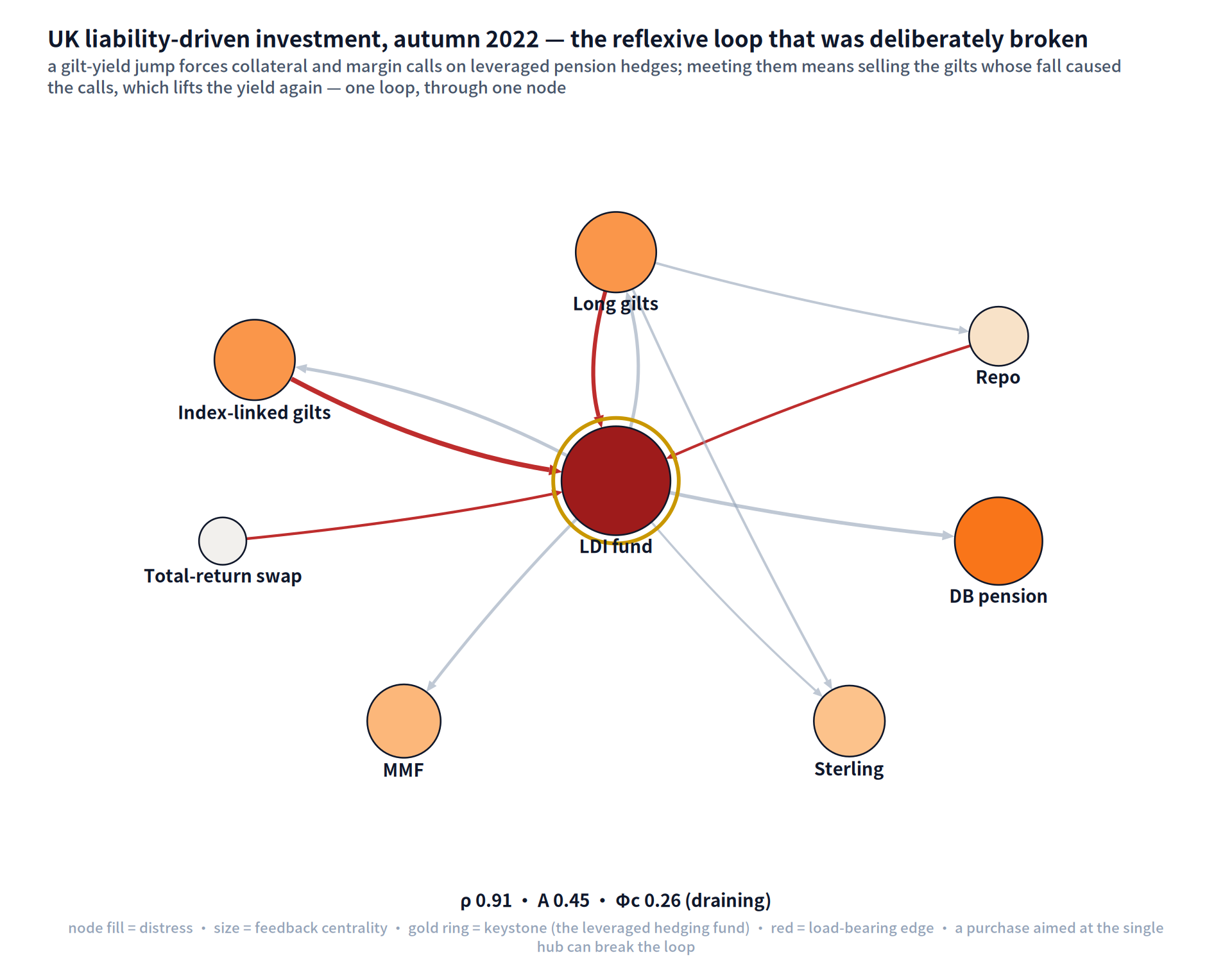
Figure 2 — UK liability-driven investment, autumn 2022. The calibrated network: the leveraged hedging fund (the keystone, gold ring) sits at the centre of a single reflexive loop running through the long-gilt market. Node fill is distress at the convergence of the cascade, node size is feedback centrality, and the red edges are the load-bearing ones. Amplification factor 0.91 (near-critical); loop concentration high; one dominant loop through one node. Computed from the calibrated network in Appendix B.

The intervention. A concentrated loop can be interrupted at a single point, and the Bank of England’s response was aimed at it. On 28 September it announced a time-limited facility to purchase long gilts, with a stated ceiling of £65 billion; in the event it bought £19.3 billion — about thirty per cent of the announced ceiling — because the announcement itself arrested the selling (Bank of England 2022; Full Fact 2022). The purchase was small relative to the gilt market, aimed at the single node the structure ran through, and, decisively, early — placed before the spiral had run its course. It is the cleanest example in the historical record of a backstop that succeeds because the loop it targets is concentrated.

The reform. What distinguishes the United Kingdom from every other case here is what followed. The Financial Policy Committee and the pensions regulator raised the resilience buffer that these funds must hold — the cushion of liquid assets that lets a fund meet collateral calls without becoming a forced seller — from around 100 basis points of yield-shock coverage before the crisis to around 300, with a 250-basis-point minimum, so that a fund can now absorb a three-percentage-point jump in real yields where it could absorb one before (Bank of England 2023; The Pensions Regulator 2024). Read through the method, the reform registers as a structural change, not a promise. The reflexive gilt-and-hedging loop that stood near the critical value on the 2022 eve now returns an amplification factor of roughly 0.61, with an early-intervention leverage of about two and a half rather than twelve (the calibration is in Appendix B; the comparison is drawn in Figure 13). The acute loop was not merely contained; the structure that produced it was reset to a lower level of amplification. This is, across the whole series, the one unambiguous case of a fragility measured, caught, and durably reduced.

That is where most accounts of 2022 stop. The structural reading does not, because the loop that was reformed is one part of a far larger centre — and the rest of that centre has not been reset.

3.2 The centre, not the instrument: London as a global complex

London is the world’s largest centre for foreign exchange, handling about 38 per cent of global turnover, and for over-the-counter interest-rate derivatives, at roughly 46 per cent (Bank of England 2022b); around four-fifths of all centrally-cleared euro-denominated interest-rate swaps are cleared through a single London clearing house (European Central Bank 2024). It is, in addition, a primary centre for offshore dollar funding; the home of the metals exchange and its clearing house, of a major energy benchmark and its clearing house, and of the world’s largest over-the-counter gold market; and the home of the insurance market that underwrites most of the world’s shipping (London Bullion Market Association 2024; London Metal Exchange 2024). We represent this complex as one network of eighteen nodes — the gilt-and-hedging core, three separate clearing houses, offshore dollar funding, foreign exchange, metals, oil, gold, insurance, the dealer banks, money funds, sterling, the central bank, and the rest of the world — with the calibration and sources set out in Appendix B.

Read through the method, the City complex returns an amplification factor of 0.88 — a range of roughly 0.84 to 0.92 under a ±20-per-cent perturbation (§2.3), and a steady-state multiplier of about eight and a half. That is well below the near-critical readings of the US Treasury and euro-area sovereign complexes, and well above the 0.61 of the reformed gilt-only network. London is not on the edge of runaway; but it is far more amplified as a whole than the one loop that was reformed. And the amplification is distributed — the loop-concentration reading is among the lowest in the entire series, close to the 2008 reading, with feedback spread across more than ninety cycles and load carried across almost all eighteen balance sheets (Appendix B; the comparison set is in Part 1). A distributed structure has no single point at which a backstop can be aimed — the property that, in 2008, made the crisis so expensive to contain.

Decompressed through Part 1’s four questions — engine, core, load, exits — the City’s map sharpens the finding rather than restating the dial. Where is the engine? The feedback spreads across ninety-four cycles, but the two strongest pairs are exactly the two bindings this section traces: the swap clearing house with the collateral pool (round-trip gain 0.16) and the dealer banks with offshore dollar funding (0.14) — the margin engine and the funding conduit — ahead of the hedge-fund–repo pair (0.10) and the gilts–LDI pair (0.08) that 2022 made famous. Which nodes form the self-reinforcing core? Thirteen of eighteen: the rates core, the dealer banks, the swap clearing house, and the entire global layer — offshore dollars, foreign exchange, sterling, gold, insurance, the foreign sector — all sit inside the block from which distress returns to its origin amplified. What sits outside is telling: the two commodity clearing houses and the Bank of England lie on one-way roads into the core — commodity margin demand injects pressure into the shared pool and never re-absorbs any. Who carries the load? No one, and that is the point: the load is the most dispersed of the three centres — an effective breadth of roughly fifteen of the eighteen balance sheets, with the heaviest single share only about eleven per cent (the repo-collateral pool, with gilts, the dealer banks, the swap clearing house and offshore dollars all within a point of it). Against the US complex, where a third of the load sits on cash Treasuries, London offers no single balance sheet to stand behind. Where would the pressure drain? Largely nowhere. The circulation fraction is 0.89 — far above today’s US complex at 0.68 — and the partition reading is one room (modularity 0.28, below the 0.3 band that marks real firebreaks, the nominal blocks heavily cross-wired). A conduit with no absorber holds what it cannot drain: the anatomical restatement of §3.4’s finding that London’s liquidity is, in the last resort, nobody’s liability.

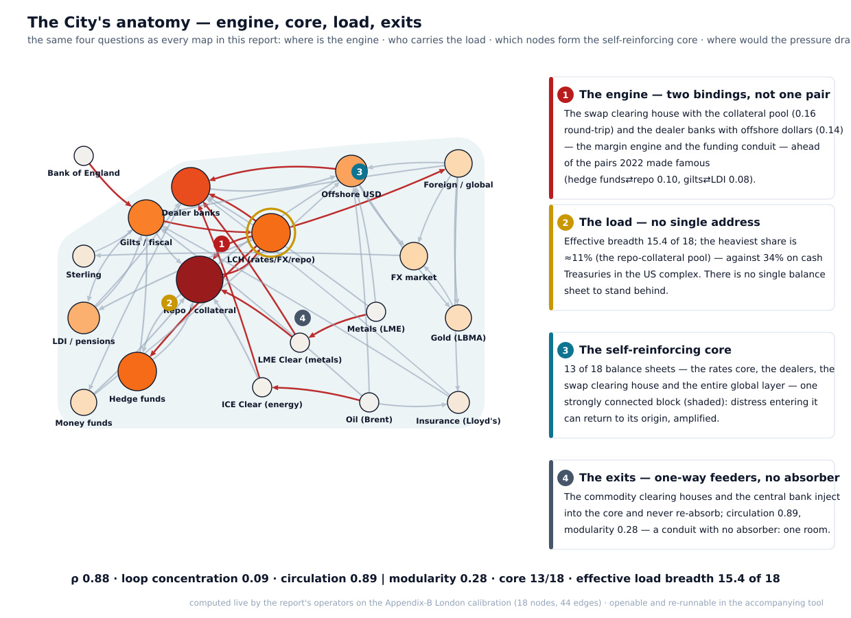
Figure 3 — The City’s anatomy, annotated: engine, load, core, exits.

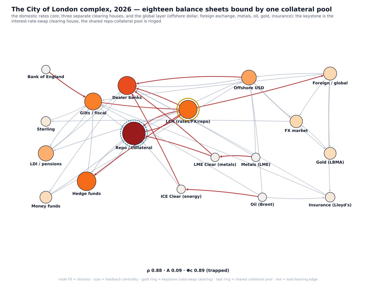
Figure 4 — The City of London complex (2026).

3.3 Why diversified clearing does not hold under stress

The single most important structural finding concerns the clearing houses, and it corrects a natural intuition. London’s clearing is separated across three central counterparties: one clears interest-rate swaps, foreign exchange and repo; a second, owned by the metals exchange, clears metals and was where the March 2022 nickel crisis occurred; a third clears energy and credit (London Metal Exchange 2024). They are legally and operationally distinct. A reasonable observer would read that separation as diversification — three independent pools of risk — and conclude that a crisis in one need not touch the others.

The network shows otherwise. The three clearing houses are bound together by two things they share: the dealer banks that are members of all of them, and the collateral and repo pool from which every one of them funds its margin. We test this directly by placing the same shock at each clearing house in turn and reading where the distress lands (Figure 5). Three results stand out. First, whichever clearing house is shocked, the dealer banks take a near-identical hit — because they are the common members. Second, a shock at the metals clearing house reaches the interest-rate clearing house even though the two are entirely separate institutions — because both draw margin from the same collateral pool. Third, the collateral pool is the most distressed node under every shock, whatever its origin. The separation of London’s clearing does not, therefore, deliver independence under stress: a metals crisis and a gilt crisis draw on the same liquidity. The two London clearing emergencies of 2022 — gilts in the autumn, nickel in the spring — were not unrelated events in different markets. They were two activations of the same shared collateral channel.

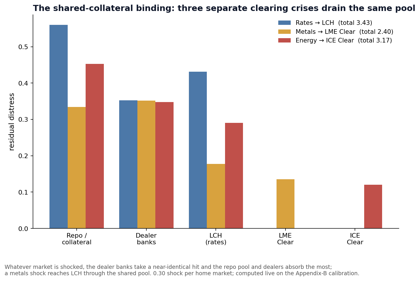
Figure 5 — The shared-collateral binding.

3.4 Liquidity in a currency the central bank cannot issue

Behind the structure is the fact that makes London different from New York. New York’s home currency is the dollar, and the Federal Reserve can issue it without limit; New York’s liquidity is, in the last resort, central-bank money. London’s home currency is sterling, but the markets it intermediates — foreign exchange, euro-swap clearing, offshore dollar funding — run on currencies the Bank of England cannot issue. London’s depth of liquidity is therefore not, in the last resort, a central-bank guarantee; it is produced by the market structure itself — by the multilateral netting that central clearing performs, which lets a member fund a net rather than a gross position; by the recycling of dollars through the repo and foreign-exchange markets; and by the depth of the dealer balance sheets that make the markets.

The network shows this as a flow signature. The offshore-dollar-funding node sits at near-balanced throughput — large flows in, large flows out — which is the signature of a conduit rather than a source or a sink: London takes in dollar liquidity and passes it on. The clearing-and-netting layer is a net source of liquidity, and the collateral pool the channel through which it moves. The corollary is structural, not rhetorical: the same features that produce London’s liquidity in calm conditions amplify distress in stressed ones. Netting frees collateral when markets are calm and calls it when they are not; the dollar conduit recycles funding when it is plentiful and transmits the squeeze when it is scarce. The capacity that makes London the world’s liquidity centre and the channel that would propagate a crisis through it are the same structure read in two conditions.

A corollary follows that bears on how this report should be read. A structure of this depth runs on global flows — offshore dollar funding, euro-swap clearing, the shared collateral pool — and not on the politics of its host, so it is largely insulated from them: the change of governing-party leadership underway in the United Kingdom through mid-2026 — a contest concluding on 17 July if unopposed, or on 29 August by members’ ballot — moves the structural reading hardly at all, because none of the load-bearing loops run through Westminster. It is the structure, not the politics of the moment, that carries the risk and that the method reads — which is also why a centre can look politically turbulent and remain structurally deep, and why the converse, a politically stable host over a migrating structure, is the more dangerous combination.

A stronger claim is warranted by the evidence. A decade of political instability — a succession of prime ministers, and a change of governing party in prospect — might have been expected to weaken London’s standing as a financial centre. The measurable outcome is the opposite: London remained the second-ranked global financial centre after New York, and was one of only two Western European centres whose rating rose in the March 2026 Global Financial Centres Index, while the euro-area venues intended to attract relocating business did not consolidate into a single competitor (Z/Yen 2026). The explanation is the one this section has developed — the depth of the centre is institutional rather than political — with one addition the rest of the series does not provide: where the supervisory response was pre-emptive, the structure was not only preserved but reduced in measured fragility. The Bank of England’s post-2022 measures are the report’s clearest instance of a supervisory response that preceded rather than followed the episode it addressed. The liability-driven-investment resilience standard lowered the reflexive loop’s amplification factor from 0.91 to 0.61 (§3.1); the Contingent Non-Bank Financial Institution Repo Facility established a non-bank lending facility that the Federal Reserve and the European Central Bank do not currently maintain (§3.5); and the system-wide exploratory scenario examined banks and non-banks jointly before a crisis required it. The reduction from 0.91 to 0.61 admits two readings: it confirms that the reform lowered the structure’s amplification, and it functions as a forward-looking indicator, in that a shock the 2022 structure would have amplified the reformed structure would now attenuate. This does not render London invulnerable — §3.5 identifies where it is not — but it is the report’s clearest case in which a fragility identified by the method was reduced by a targeted and early intervention.

3.5 The backstop toolkit and the gap

The Bank of England is not unprepared, and this report does not suggest it is. It has built a deliberate, graded set of facilities, and it widened that set precisely in response to 2022. Banks can obtain sterling liquidity through the short-term and long-term repo operations and the discount window, against collateral that is being progressively widened (Bank of England 2025). Banks can obtain dollars through the standing swap line the Bank holds with the Federal Reserve — part of the six-central-bank swap network made permanent in October 2013 — and, if needed, through the Federal Reserve’s repo facility for foreign authorities (Federal Reserve 2013; Federal Reserve 2020). And, most tellingly, non-banks — pension funds, liability-driven investment funds, insurers — can now borrow sterling directly against gilts through the Contingent Non-Bank Financial Institution Repo Facility, opened to applications in January 2025, a direct institutional answer to the 2022 crisis that extends the backstop to the very institutions that propagated it (Bank of England 2024).

Mapped against the network, this set of facilities is organised along two of our reachability dimensions — bank versus non-bank, sterling versus dollar — and it covers most of the grid. The swap line covers banks in dollars; the repo operations and discount window cover banks in sterling; the new non-bank facility covers non-banks in sterling against gilts. What it does not directly cover is the one combination the network flags as the rising vulnerability: non-banks, in dollars, and the cross-clearing-house collateral spiral. We grade the two halves of that gap by the strength of their evidence, because they are not equally established.

The non-bank dollar half is backed by data and is, on the evidence, a vulnerability that is currently rising. The cash-futures basis trade — leveraged funds holding cash government bonds against short futures, funded in repo — reached roughly $1 trillion of net short positions in Treasury futures of up to ten-year maturity by March 2025, a record, and well above the level on the eve of the March 2020 dash-for-cash (Federal Reserve 2024; Federal Reserve 2025). Cayman-domiciled funds, managed substantially out of London and New York, held $1.85 trillion of Treasuries — up about a trillion since 2022 — with repo borrowing of $2.5 trillion in the fourth quarter of 2024, a 104-per-cent rise in two years, and the largest funds running at leverage above eighteen to one (Federal Reserve 2025). In the United Kingdom specifically, hedge-fund net repo borrowing in the gilt market stands at its highest since records began in 2016, with seven funds accounting for ninety per cent of it (Bank of England 2025b). The Financial Stability Board’s 2025 report on non-bank leverage names government-bond-market leverage and the basis trade as systemic concerns (Financial Stability Board 2025). This is a dollar exposure, run by non-banks, intermediated through London — and the swap line reaches the banks that fund these non-banks only indirectly, through dealer intermediation that, in March 2020, broke down badly enough that the Federal Reserve had to buy roughly $1 trillion of Treasuries directly. Bank dollar liquidity is necessary; the 2020 precedent shows it is not sufficient for a non-bank, market-functioning seizure.

The cross-clearing-house collateral half is established as a mechanism but is not, on the evidence we have, a rising trend, and we present it as such. That central-counterparty margin is procyclical — that it rises with volatility, drains liquidity exactly when liquidity is scarce, and transmits through the banks that are common members and common contributors to default funds — is a documented systemic concern (Federal Reserve 2020b; World Federation of Exchanges 2021). The 2022 nickel crisis is the worked example, and the network locates the channel structurally, through the shared collateral pool (Figure 5). What we do not have is a time series showing commodity-clearing margin demand currently rising the way the basis trade is. We therefore make the structural claim — that the separate clearing houses are bound to the rates-and-repo core by a shared collateral pool, a binding the 2022 episodes demonstrated — and we do not present it as a trend.

That these are the gaps is not our assertion alone; they are the frontier the authorities themselves are working on, which is why the point can be made without alarmism. The Bank of England’s discussion paper on gilt-repo resilience and its 2026 feedback statement, its consultation on the resilience of clearing houses, its supervisory stress test of the three UK central counterparties, and — most directly — its System-Wide Exploratory Scenario, the first such exercise anywhere to model banks and non-banks together under the same stress, all address exactly this territory; the scenario reported that the post-2022 reforms had improved gilt and gilt-repo resilience, but that a dynamic of procyclically rising repo haircuts remains a live concern (Bank of England 2024b; Bank of England 2025; Bank of England 2026). The policy response so far, though, is largely preventive — higher margins and haircuts, liquidity preparedness, and a sterling-against-gilts facility for non-banks now onboarding its first participants — rather than a lender of last resort for the non-bank-dollar and cross-clearing-house channels the network flags. The boundary of the toolkit and the location of the keystone differ by exactly this combination.

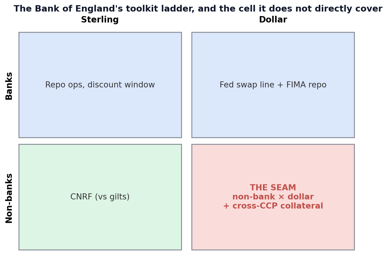
Figure 6 — The toolkit and the gap. Counterparty (bank / non-bank) against currency (sterling / dollar), with the Bank of England’s facilities placed on the grid: the repo operations and discount window (bank, sterling); the Federal Reserve swap line and the foreign-authority repo facility (bank, dollar); the Contingent Non-Bank Financial Institution Repo Facility (non-bank, sterling, against gilts). The uncovered cell — non-bank, dollar — together with the cross-clearing-house collateral spiral, is the residual gap.

4. The euro area: a powerful central bank without a common treasury

4.1 The reference crisis: the sovereign–bank loop of 2010–12

The euro area’s reference crisis differs from every other case in this series in the character of its loop. The crises of 1929, 2008, the 2020 dash-for-cash and the 2022 gilt episode were liquidity spirals — forced sellers meeting collateral calls, a shortage of cash against fundamentally sound assets. The euro-area crisis of 2010–12 was a solvency spiral, in which the feedback ran not through a margin account but through the capital of banks and the debt of states (the calibration, carried from Part 1’s European material, is in Appendix B).

The loop. The mechanism had four legs, and each fed the next. A peripheral sovereign — Greece, then Ireland, Portugal, Spain and, decisively, Italy — saw its borrowing cost rise. Domestic banks, which held large quantities of their own government’s bonds, took losses on those holdings, eroding their capital. Weakened banks contracted lending to the real economy and, where they needed support, drew on their sovereign for recapitalisation or guarantees — which added to that sovereign’s debt. The heavier debt, the weaker economy and the impaired banks pushed the sovereign’s borrowing cost higher still, and the loop closed. A ratings channel ran alongside it: each downgrade of the sovereign mechanically pressured its banks and widened the haircut on the bonds they pledged for funding, tightening the squeeze.

The public record. The episode left an unusually clear trail. Italian ten-year yields reached 7.26 per cent in November 2011 and Spanish yields 7.6 per cent in July 2012 — levels widely judged unsustainable for sovereigns of that size. The European Central Bank’s two long-term refinancing operations injected roughly €1.02 trillion of three-year bank funding across December 2011 and February 2012; the Greek private-sector debt restructuring of March 2012 wrote down privately-held bonds at a 53.5-per-cent haircut; and the imbalances in the euro-system’s internal payment system reached approximately €1 trillion at their 2012 peak — a measure of how far private capital had fled the periphery for the core (the public anchors are listed in Appendix C).

The network reading. Represented as a network — peripheral sovereign debt, peripheral banks, foreign investors, wholesale funding, the ratings channel and the real economy — the 2010–12 structure returns an amplification factor of 0.97, with a range of roughly 0.91 to 1.03 under a ±20-per-cent perturbation, the highest near-critical reading among the historical European cases (Appendix B). As in the 2022 case the loop is concentrated and the keystone is robust: in every perturbation draw the node carrying the most feedback is peripheral sovereign debt, and the four loops — solvency, ratings, foreign exit, wholesale funding — all cross that single hub (Figure 7). The early-intervention leverage is roughly thirty-five: at this degree of amplification the premium on acting early rather than late is extreme.

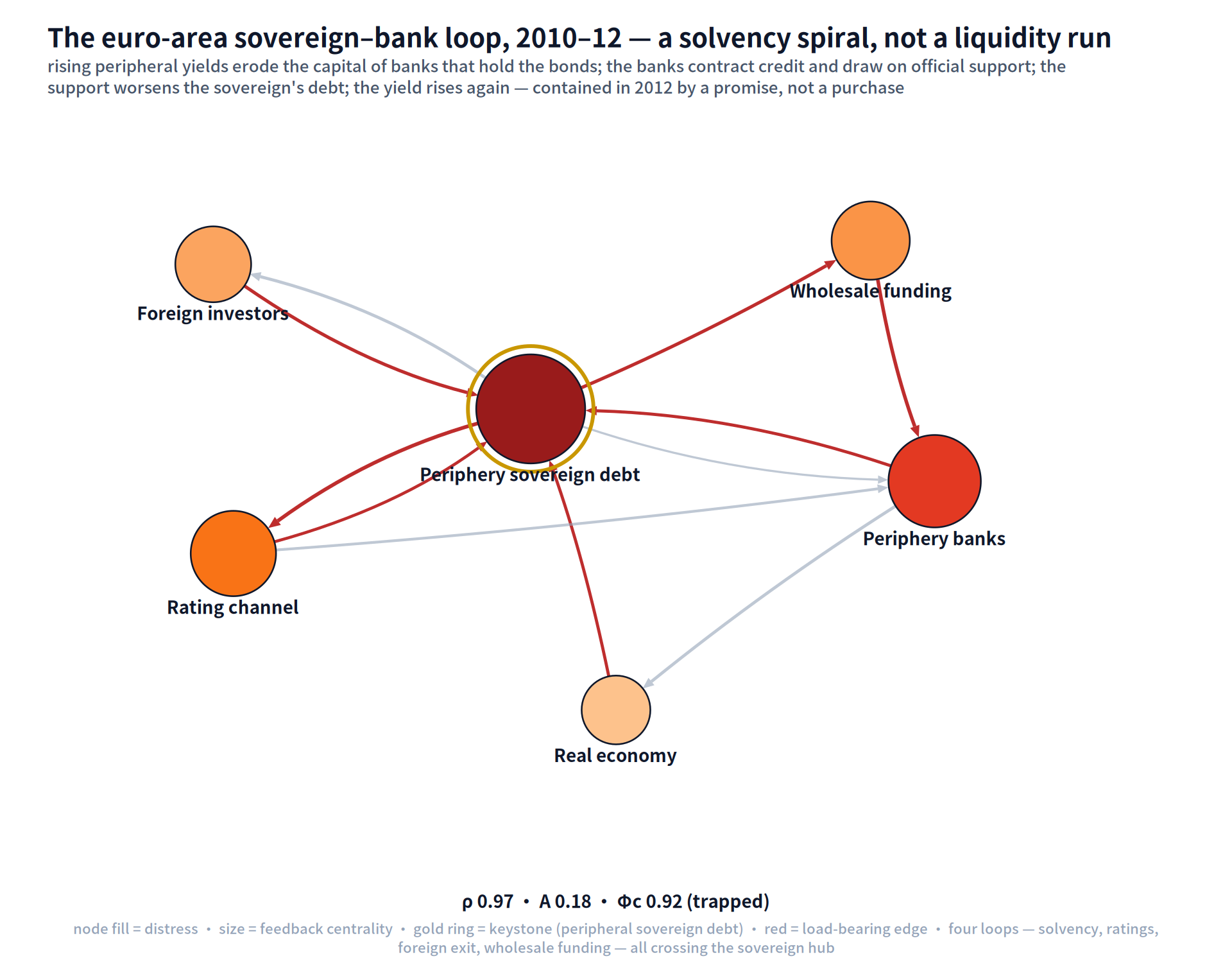
Figure 7 — The euro-area sovereign–bank loop, 2010–12.

Containment by commitment. What contained the crisis is the most distinctive intervention in the historical record, and it is central to this Part’s argument. In July 2012 the President of the European Central Bank stated that the bank would do “whatever it takes” to preserve the euro; the statement was operationalised as Outright Monetary Transactions, a facility to purchase a member state’s bonds in the secondary market (European Central Bank 2012). Peripheral spreads compressed sharply — and not a single bond was ever bought under the facility. It worked entirely through the credibility of the commitment. It is the purest example in this series of containment by commitment rather than by purchase: where the Federal Reserve in 2020 and the Bank of England in 2022 had to buy, the European Central Bank in 2012 only had to promise convincingly. Its successor instrument, the Transmission Protection Instrument announced in 2022, has the same character and has likewise never been activated (European Central Bank 2022).

The dual outcome. One feature of the episode anchors a finding that recurs across the series: containment determines the outcome. The same crisis produced two very different results, depending on whether the backstop reached. The core and the larger periphery, brought inside the commitment, suffered a deep but bounded recession — euro-area output fell about 1.5 per cent peak to trough. Greece, where the adjustment was largest and the backstop least able to reach a sovereign already in restructuring, lost more than a quarter of its real output cumulatively, an outcome on the scale of the 1930s. The structure was one; the outcomes diverged with the reach of the backstop.

4.2 The euro area today: near-critical again, and migrating

Read today, the euro-area sovereign-bank structure returns an amplification factor of 0.96 — near-critical, close to the 2012 crisis reading itself, in a period of compressed spreads and market calm. The structural tension has returned while prices are quiet: the same finding as the US case, in a European register. But the more important reading is a migration. In 2012 the structure was a set of distributed loops running through a single sovereign hub — Italy — so that one backstop, aimed at that hub, could in principle catch the whole. Today the keystone reading has slipped from a single-hub value to one in which a second sovereign — France — carries roughly a tenth of the feedback, and carries it outside the Italian hub (Appendix B).

The same four questions, put to the euro-area map, return the starkest anatomy in the series. The engine: nineteen cycles, led not by the domestic bank–sovereign pair but by the foreign-exit loop — Italian debt with its non-resident investors, at a round-trip gain of 0.23 — ahead of the banks–sovereign–wholesale funding triangle (0.12), the direct bank–sovereign pair (0.10) and, new against 2012, a France–Italy sovereign pair (0.075): a loop that did not exist when the periphery was only the periphery. The core: six of seven nodes — everything except the central bank’s quantitative-tightening node, which sits on a one-way road into the loop: in today’s wiring the official sector injects pressure, as a seller, and absorbs none. The load: the two sovereigns together carry forty-six per cent of total exposure — Italy twenty-eight, France eighteen — with the banks at seventeen; unlike London’s, the euro area’s load axis has clear addresses, and they are the two bond markets §4.3 shows the backstop reaching only conditionally. The exits: there are none. The circulation fraction is 0.93, the highest of the three centres, and the partition reading is the lowest in the whole series at 0.07 — every crisis-eve network in Part 1 read at least 0.11 — making the euro-area complex the most nearly one-room structure in the record. A solvency loop with no absorbing node is exactly the structure that containment-by-commitment repaired in 2012, when the commitment grafted an absorber onto a network that had none; it is also exactly the structure on which today’s graft is conditional (§4.3), while the official node, under quantitative tightening, works as an injector.

The engine’s real-world counterpart is directly observable in the holding structure. Non-residents hold 53.8 per cent of France’s standard bonds — and 82.9 per cent of its short-term bills — against roughly 31 per cent of Italy’s securities, where a deliberate retail programme has raised household holdings to about 15 per cent (Agence France Trésor 2026; Scope Ratings 2025). The foreign-exit loop the operators rank first is therefore largest, in holding-structure terms, precisely at the sovereign into which §4.2’s keystone reading says the fragility is migrating; Italy, the hub, has meanwhile been rebuilding the domestic buffer that dampens that engine.

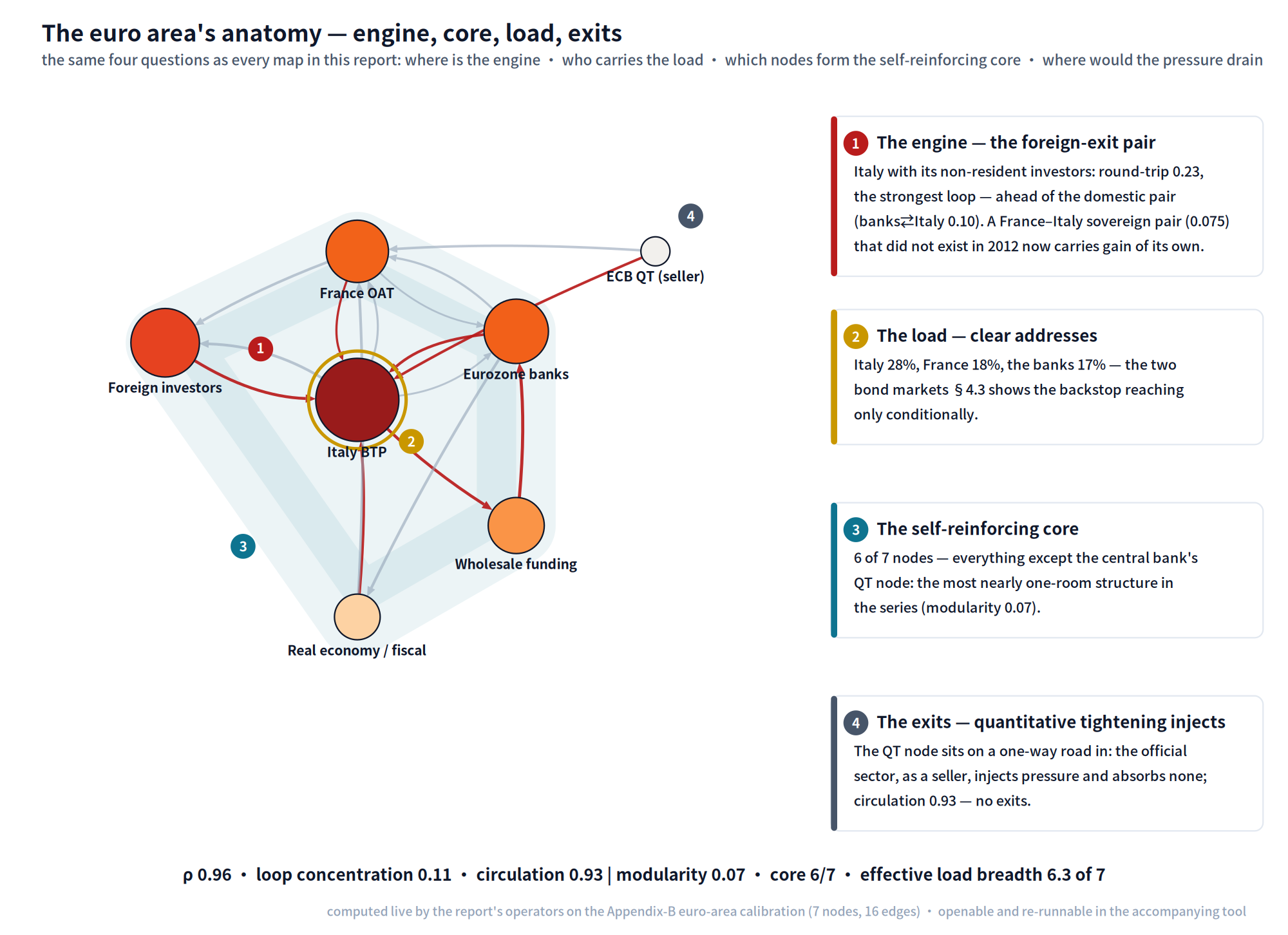
Figure 8 — The euro area’s anatomy, annotated: engine, load, core, exits. The seven-node euro-area network with the self-reinforcing core shaded, read through the same four questions. ① The engine is the foreign-exit pair — Italian debt with its non-resident investors (round-trip gain 0.23) — ahead of the domestic bank–sovereign pair; a France–Italy sovereign pair (0.075) that did not exist in 2012 now carries gain of its own. ② The load has clear addresses: Italy 28 per cent, France 18, the banks 17. ③ The core spans six of seven nodes — the most nearly one-room structure in the series (modularity 0.07). ④ The quantitative-tightening node feeds it one-way: the official sector injects, as a seller, and absorbs nothing; circulation 0.93.

France has become a second centre of fragility, and through a route worth stating precisely, because it bears on the policy question in §4.3. The pressure is not a single fiscal miss: France’s public deficit came in at 5.1 per cent of GDP in 2025, in fact below the level that had been feared and down from 5.8 per cent in 2024 (Insee 2026). It is, rather, a matter of trajectory and governability. French public debt reached 115.6 per cent of GDP at the end of 2025 and is projected to keep rising through the rest of the decade on official and IMF projections, with no stabilisation in sight (Insee 2026; IMF 2025); and a succession of governments through 2024–25 — two of them brought down by the budget — put the country’s capacity for sustained fiscal adjustment in question. The minority government that emerged did pass a deficit-reducing 2026 budget in February 2026, but only narrowly, on contested concessions and against repeated no-confidence motions, which is the more telling fact: France can still legislate an adjustment, but each one is bought at the cost of the governing coalition’s stability (Al Jazeera 2026). And the European Central Bank, which was the buyer of last resort in 2012, is today a seller, reducing its balance sheet through quantitative tightening — the backstop is stepping back as the structure tightens (European Central Bank 2024b).

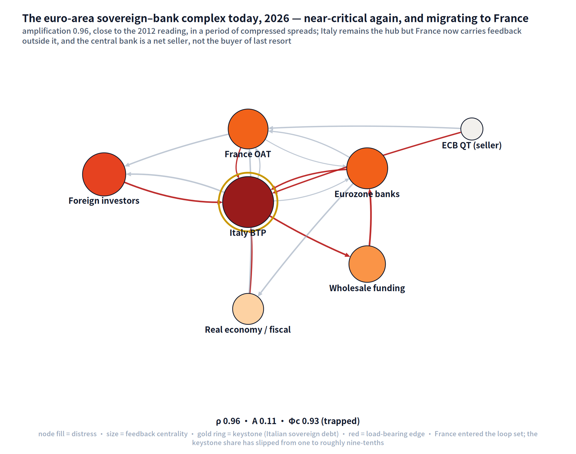
Figure 9 — The euro area today (2026). The sovereign-bank network reads an amplification factor of 0.96 — near-critical, close to the 0.97 of the 2012 crisis itself — but with France now in the loop set and carrying feedback outside the Italian hub: the keystone share has slipped from one (2012) to roughly nine-tenths as France entered, and the European Central Bank is now a net seller (quantitative tightening), not the buyer of last resort.

4.3 The conditionality question: when can the backstop fire?

The euro area’s containment tool is conditional, and the report’s core policy contribution is to make the conditionality concrete and then to simulate it. The Transmission Protection Instrument can be activated only if the member state meets four eligibility conditions, the first of which is compliance with the European Union fiscal framework — including not being under an excessive-deficit procedure without having taken effective action on the Council’s recommendations (European Central Bank 2022). France is under an excessive-deficit procedure, with a Council-recommended adjustment path (Council of the European Union 2025). Being in the procedure does not automatically disqualify it; eligibility turns on whether France is taking effective action on the path. And that is exactly what the political instability of 2024–25 — the succession of governments, the difficulty in passing a budget — puts in question, even though the 2025 deficit itself came in better than feared. Eligibility turns not on a single year’s number but on the credibility of sustained adjustment, and that is what the instability erodes. The result is a structural paradox, now grounded in fact: France’s eligibility for the backstop depends on the fiscal-political credibility that a crisis would itself erode — the tool is least available to the sovereign that has become the centre of the fragility, at the moment it would be most needed.

We simulate the question on the calibrated network, with the simulation defined in Appendix A. Three results matter, and a fourth qualifies them.

• When a shock originates at France and the backstop is blocked — conditionality excludes it — the network reaches the highest total distress of any scenario in the set, higher than an unrescued Italian shock, because France roughly doubles the loop count.

• When the central bank intervenes by purchasing the Italian keystone — the periphery the instrument was built for — a France-originated shock is substantially contained at the system level, because most of the cascade routes through the Italian hub; but France’s own bond market is left carrying the highest residual distress in the network, because the purchases are not aimed at it. Defending the hub protects the system, not the origin.

• When the central bank instead purchases French bonds directly, France’s own residual distress falls the most, but the system-wide containment is weaker than defending the hub — a genuine structural trade-off between protecting the system and protecting the stressed member.

• The qualifier is timing. The euro area’s higher amplification means the premium on acting early is larger than the United Kingdom’s: the early-intervention leverage is roughly 27 for the euro area against roughly 12 for the 2022 gilt structure (Figure 13). A small, early, well-aimed purchase contains the spiral; the same purchasing power applied late barely moves it. The tension is acute: the euro area needs speed more than the Bank of England did, and its conditionality framework — verifying eligibility, judging whether stress is fundamentals-driven — is precisely what introduces delay (the supporting sweep is in Appendix B).

The policy reading for the decision-maker is therefore not “the instrument is too small.” It is that any activation beats none by a factor of two to three; that the structurally optimal purchase target for system-wide containment is the hub, not the origin; and that the binding constraint is the conditionality assessment, which is slowest exactly where the structure makes delay most costly.

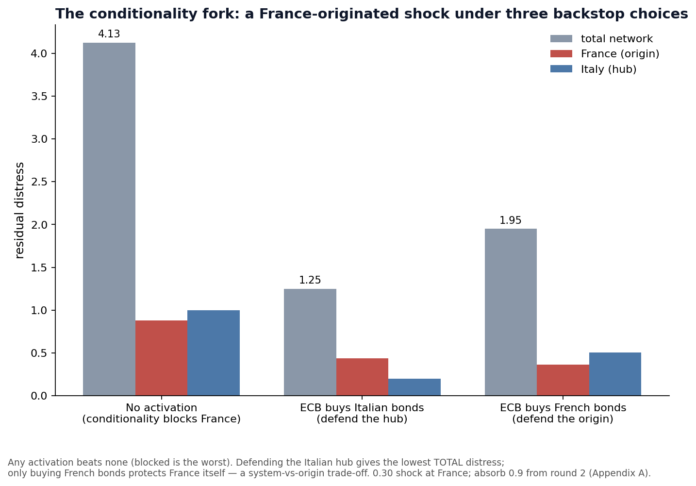
Figure 10 — The conditionality question. Residual distress under a France-originated shock for three backstop choices: no activation (conditionality blocks France) — the worst outcome in the set; purchase of the Italian hub — lowest total distress, because the cascade routes through Italy, but France’s own market is left carrying the most; purchase of French bonds — protects France itself at the cost of weaker system-wide containment. Any activation beats none by a factor of two to three. Reproducible by varying the backstop target on the calibrated euro-area network in Appendix B.

4.4 A polycentric centre and a differently-shaped gap

The euro area’s containment gap is often misread as a weakness of its central bank. It is not. The European Central Bank can issue euros without limit; on the currency dimension of reachability it is in the same position as the United States and a stronger position than the United Kingdom, which cannot issue the dollars London runs on. The gap is in the two dimensions a central bank, however powerful, cannot fill on its own.

The first is the missing fiscal union. A unitary state backstops its own debt unconditionally — the Bank of England bought gilts in 2022 without conditioning on the United Kingdom’s fiscal compliance, because it is the central bank for its own sovereign’s debt, indemnified by its own treasury. The European Central Bank buying a member’s bonds is taking on that member’s credit risk with no common treasury to share it, which is the root reason — together with the Treaty prohibition on monetary financing — that the sovereign backstop must be conditional in the first place (European Central Bank 2022). The conditionality is not a design flaw to be corrected by the central bank; it is the consequence of the absent fiscal union.

The second is fragmented supervision over a polycentric structure. Where New York and London concentrate their venues and their infrastructure in one city under one supervisor, the euro area’s financial functions are dispersed — Frankfurt took much of the banking, Paris a mix, Dublin and Luxembourg the asset managers, Amsterdam the trading venues — in a post-Brexit redistribution that moved more than £900 billion of bank assets and produced not a new single hub but a set of specialised centres (New Financial 2021). That dispersion reads, at first glance, as diversification. But it is bound, as London’s clearing houses are bound, by shared infrastructure — a common securities-settlement layer, a few large depository groups, the same clearing houses — across which the European Central Bank and the Single Supervisory Mechanism oversee the large banks while much of the market infrastructure remains supervised by national authorities, with the central bank itself calling the resulting fragmentation an urgent problem (European Central Bank 2025). The dispersion of the union’s centres delivers, structurally, the same kind of false comfort as the separation of London’s clearing: venues that look independent, bound by shared infrastructure and overseen by no single authority that can see or backstop the whole.

Two measured readings confirm that the dispersion is not consolidating into a rival, and that the liquidity between the centres runs core-ward (Figure 11). The first is competitiveness: in the Global Financial Centres Index of March 2026, of all the Western European centres only London and Madrid improved their ratings, Amsterdam displaced Dublin from the global top twenty, and the euro-area venues otherwise slipped — while Zurich and Geneva, both outside the euro area, out-rank every euro-area venue but none of them forms a rival either: a set of specialised centres trading places, not a single competitor forming (Z/Yen 2026). The second is the liquidity itself: the euro-system’s internal TARGET balances stand at roughly €1.07 trillion of Bundesbank claims against the debtor positions of the periphery — Italy near −€360 billion, Spain near −€450 billion, and, tellingly, France now among the debtors at about −€190 billion — the same flight of private capital from periphery to core that the 2012 crisis produced, and the same core-ward drift the migration of §4.2 describes, visible here as a creditor centre and a debtor rim (European Central Bank 2026).

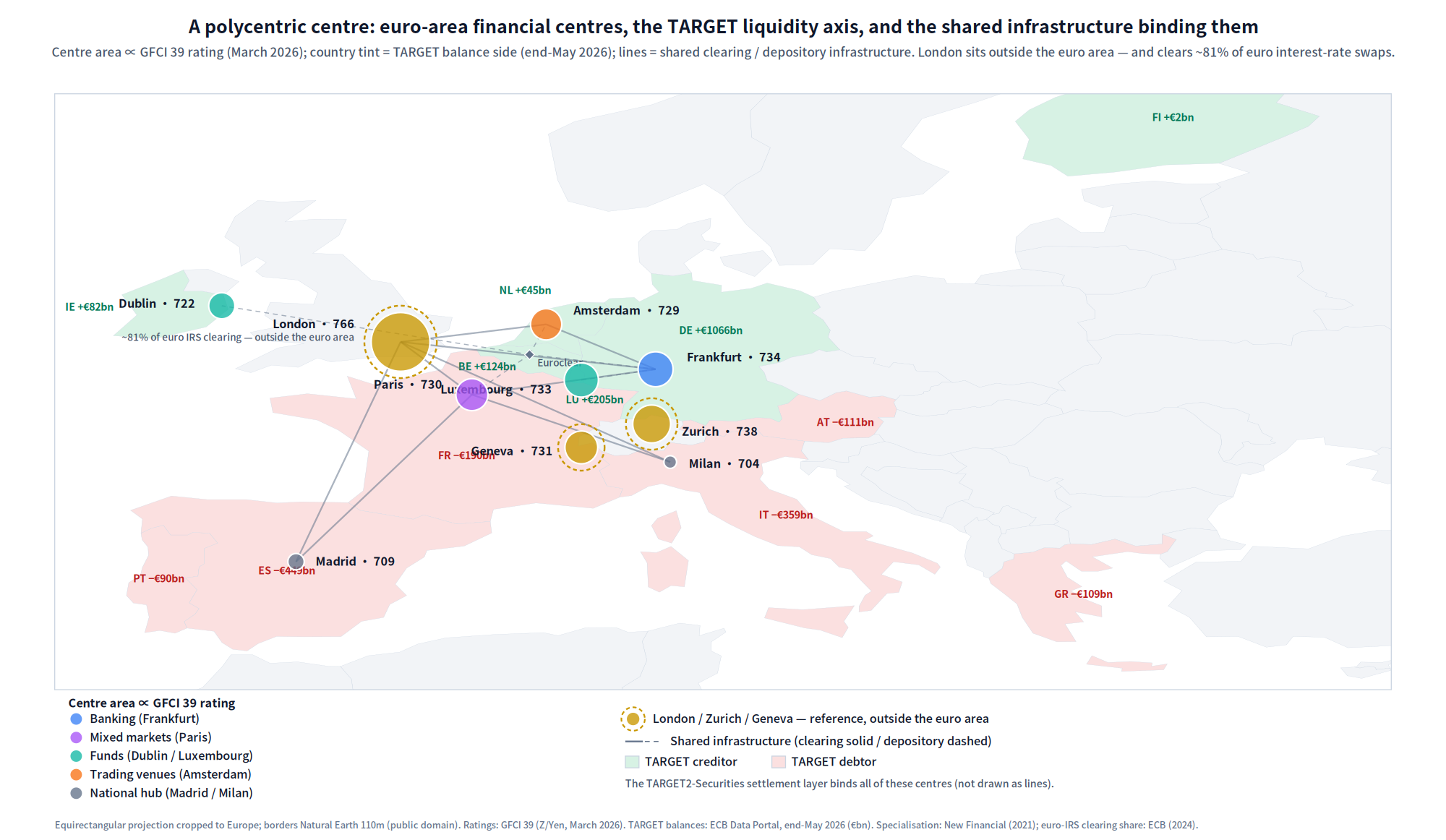
Figure 11 — A polycentric centre. The euro-area financial centres, sized by their March 2026 Global Financial Centres Index rating and coloured by post-Brexit specialisation (Frankfurt banking, Paris mixed, Dublin and Luxembourg funds, Amsterdam venues, Madrid and Milan national); country tint marks the TARGET-balance side at end-May 2026 — creditor core (green) against debtor periphery (red), with France among the debtors; the lines are the shared clearing and depository infrastructure that binds the “separate” centres. London, Zurich and Geneva are ringed outside the euro area: London still clears roughly 81 per cent of euro interest-rate swaps, and Zurich and Geneva both out-rank Frankfurt. Sizes, balances and bindings are the same constants the accompanying tool’s euro-area lens reads. Sources: GFCI 39 (Z/Yen 2026); ECB Data Portal TARGET balances (European Central Bank 2026); New Financial 2021; European Central Bank 2024.

There is a sharp, specific instance of the dependency. The European Union has, since Brexit, pursued “strategic autonomy” in clearing — moving euro-denominated derivatives clearing from London to Frankfurt — and has largely not achieved it: euro interest-rate-swap clearing remains roughly 81 per cent in London against 19 per cent in Frankfurt, because London’s multi-currency clearing house lets members net across currencies and so post far less collateral than a single-currency alternative would demand (European Central Bank 2024; London School of Economics 2025). The netting economics that make London the cheaper place to clear are the same economics that bind its clearing houses together; and they leave the euro area structurally dependent, for the clearing of its own currency, on a centre outside its jurisdiction and its backstop. The union’s gap is not that its central bank is weak. It is that the union cannot, by construction, backstop unconditionally — and cannot, in practice, even repatriate the clearing of its own currency.

5. Three centres, three gaps

The three centres are best compared not by how fragile they are — all three read near or above their historical danger marks — but by where their backstop runs out (Figure 12). The shape of the gap is the variable that decides how each would break, and what it would take to catch.

The reading runs across the row. New York is the benchmark of a complete backstop — its currency, its sovereign debt and its supervision all sit inside one reach, which is the privilege Part 1 measured. London can backstop its own currency and supervises its own infrastructure under one authority, but it borrows the currency it runs on, and its load-bearing exposures have migrated to the one combination — non-banks, in dollars, through the clearing collateral pool — that its toolkit reaches only indirectly. The euro area can issue the currency it runs on, but cannot backstop its members unconditionally and cannot supervise its dispersed infrastructure under one authority — so its gap is the sovereign conditionality and the fragmentation, not the currency.

None of the three is “safe,” and none is simply “more fragile” than the others. They would break in different places, and a backstop designed for one would miss the gap of another. That is the practical payoff of reading them through reachability rather than through a single fragility score: it tells the policymaker not how worried to be, but where an intervention would have to be made, and whether any existing facility can make it.

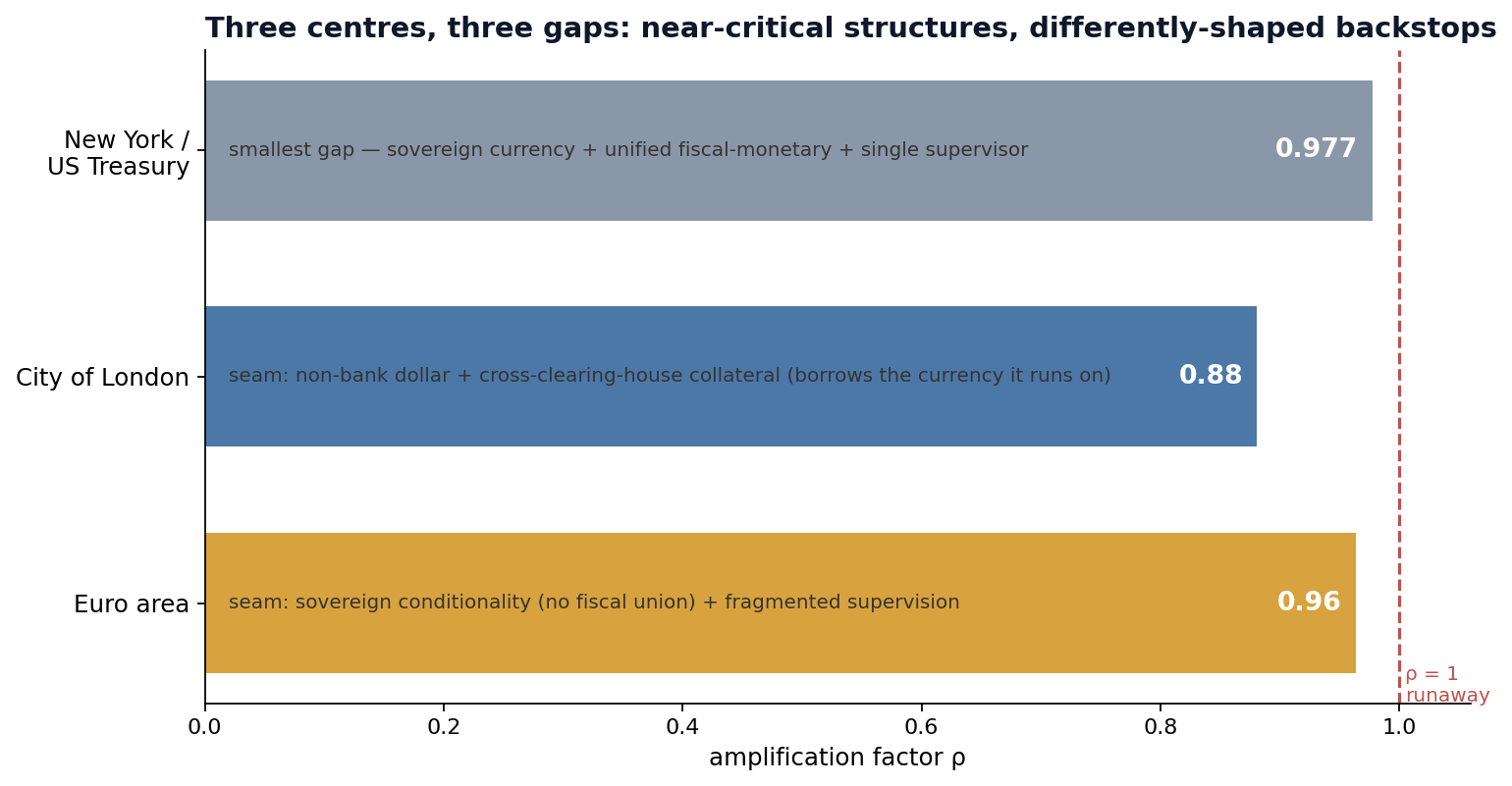
Figure 12 — Three centres, three gaps. Amplification factors for the US Treasury complex (0.977), the City of London (0.88) and the euro area (0.96), each annotated with the location of its backstop gap. Three structures near or above the historical danger marks, with three differently-shaped backstop boundaries — the smallest gap (New York), the borrowed-currency gap (London), and the no-fiscal-union gap (the euro area).

The amplification factor also carries a direct operational reading, shown in Figure 13: the value of catching a spiral early rises steeply as a structure approaches criticality. The early-intervention leverage — the steady-state multiplier, one divided by one minus the amplification factor — runs from about two and a half for the reformed UK gilt complex to roughly forty for the US Treasury complex. It is the single clearest summary of why the United Kingdom’s 2022 reform matters: by cutting the gilt-and-hedging structure’s amplification factor from 0.91 to 0.61, it cut the leverage on acting early from about twelve to about two and a half — the one structure in the set that was deliberately moved away from the threshold.

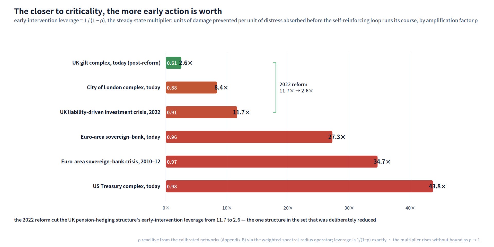
Figure 13 — The value of acting early, by amplification factor. Early-intervention leverage, one divided by one minus the amplification factor, for each case: the units of damage prevented per unit of distress absorbed before the loop runs its course. The multiplier rises without bound as the amplification factor approaches 1; the 2022 UK reform is the one move down the ladder (11.7 to 2.6). Amplification factors read live from the calibrated networks in Appendix B.

5.1 The three centres coupled: a first structural reading

The comparison above treats the three centres as three systems. They are not. The channels that join them are documented, large, and already load-bearing in this report: London’s offshore-dollar funding is the conduit for the dollars New York’s repo market supplies (§3.4); the basis books that hold a record short position in Treasury futures are managed substantially out of London (§3.5); roughly 81 per cent of euro interest-rate swaps clear through a London clearing house whose margin calls land on euro-area banks (§4.4); and United States money funds are a standing wholesale funder of both London’s dealer banks and the euro area’s banks — the channel whose withdrawal in 2011 forced euro-area banks out of dollar lending (Ivashina, Scharfstein and Stein 2015) — and an intermediation chain the European Central Bank’s November 2025 Financial Stability Review describes in exactly the form drawn here: euro-area global banks sourcing funding from United States money funds and on-lending it, secured, to hedge funds (European Central Bank 2025b). We therefore close with a first structural reading of the three as one system: the three published calibrations, joined by ten cross-centre edges — one per documented channel, weighted by mechanism class within the same ranges as Appendix B, and not tuned to any target.

The reading is stated in one line and then qualified honestly. Each centre alone is below the runaway threshold; the coupled system is above it. Individually the three return amplification factors of 0.88, 0.96 and 0.977. Joined by the ten documented channels, the coupled system returns 1.11. The result is robust in the direction that matters: with every cross-centre edge set at the conservative low end of its mechanism class the coupled reading is still 1.07, and under a ±30-per-cent perturbation of the cross-centre edges alone, every one of two thousand draws remains above 1 (Figure 14). How weak the coupling would have to be for the reading to fall back below the threshold is answered directly, in an observable coordinate, in §5.4 (Figure 16): the critical funding state sits far below any normal one. Two further checks bound the claim. Removing any one of the ten channels — or any two jointly — leaves every reading above 1 (leave-two-out minimum 1.02). And a null model that keeps the ten weights but rewires their endpoints at random across the blocks crosses the threshold in 63 per cent of draws: coupling three near-critical structures is generically destabilising, which is itself part of the finding — while the documented wiring reads above the null’s 95th percentile, so the real channels amplify more than random ones. The claim is therefore a model reading, not a market observation: under the stated coupling calibration, the coupled system is model-supercritical. What the reading means is what §2.4 says such readings mean, no more: not that runaway is underway — it visibly is not — but that the coupled structure, unlike each of its parts, would not damp a shock by itself. Within each centre, the structure attenuates; between them, it amplifies. What holds the whole is therefore not the structure but the backstops — and the backstops are national, while the amplification is not.

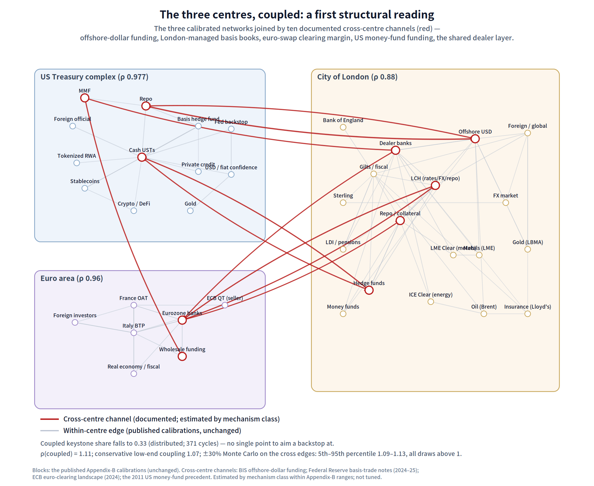
Figure 14 — The three centres, coupled: a first structural reading. The three calibrated networks of this report joined by ten documented cross-centre channels (red) — offshore-dollar funding, London-managed basis books, euro-swap clearing margin, US money-fund funding, the shared dealer layer; block calibrations unchanged from Appendix B. Coupled reading 1.11 (conservative 1.07; ±30% Monte Carlo on the cross edges: 5th–95th percentile 1.09–1.13, all draws above 1).

The second reading is the shape. Each centre alone has an identifiable keystone — cash Treasuries, the swap clearing house, the Italian sovereign — a single place a backstop can aim. In the coupled system the keystone’s share of cycle gain falls to a third, the loop-concentration reading turns distributed, and the feedback spreads across some 370 cycles: the coupled system has the 2008 shape, the kind that is expensive to contain because there is no single node to defend (§3.2). And the institutional map matches the structural one: no authority spans the three centres, and the one standing cross-centre instrument is the swap-line network, which supplies dollars to banks — precisely the channel the non-bank dollar exposure of §3.5 bypasses.

Part 1’s remaining lenses complete the reading. The circulation fraction of the coupled system is 0.79: distress placed anywhere returns through the network’s loops rather than draining to an absorber — between the US complex alone (0.68) and the European blocks (0.89 and 0.93), so the coupling opens no exit that the parts lacked. The load axis disperses as the feedback axis does: exposure spreads across an effective breadth of roughly twenty-nine of the thirty-seven balance sheets, with a concentration index of 0.04 — the coupled system does not even have the single most-loaded node that Part 1 found in today’s US complex, where cash Treasuries carry a third of total exposure. On both of Part 1’s axes, feedback and load, this is the 2008 shape, one level up.

The anatomy adds the one finding in this series that changes what containment could mean. The self-reinforcing core — the set of balance sheets from which distress can return to its origin amplified — spans twenty-seven of the thirty-seven nodes and crosses all three centres: the core crosses borders, while every authority stops at one. Yet the partition reading, alone in the whole series, is strong: a modularity of 0.54, against a historical record in which no crisis-eve network reached 0.3 (the COVID network read 0.11) — and the three communities the partition finds are exactly the three centres. Part 1 observed that no pre-crisis network has internal firebreaks, and that every successful containment in the record was an external graft rather than an internal boundary holding. The coupled system is the first structure in the series that has internal boundaries — and they are precisely the ten cross-centre channels. The topology, in other words, contains the partitions a containment policy would need; but the control points on those boundaries — the margin gates at the clearing seam, the swap-line network at the funding seam — sit across institutional jurisdictions, held by no single authority.

The cascade reading makes the propagation concrete. A shock seeded at the French sovereign saturates London’s hedge-fund and repo-collateral complex and, through the basis books, cash Treasuries themselves — the distress arrives at the other two centres through exactly the channels the partition identifies as the boundaries. The periphery this system drives, from Asia to Latin America, and cross-centre edges calibrated in full from flow data lie beyond this report’s scope; but two steps are available now, and §5.4 and §5.5 take them — replaying the record’s actual crossings on this frozen network, and letting each edge move with the observables already public.

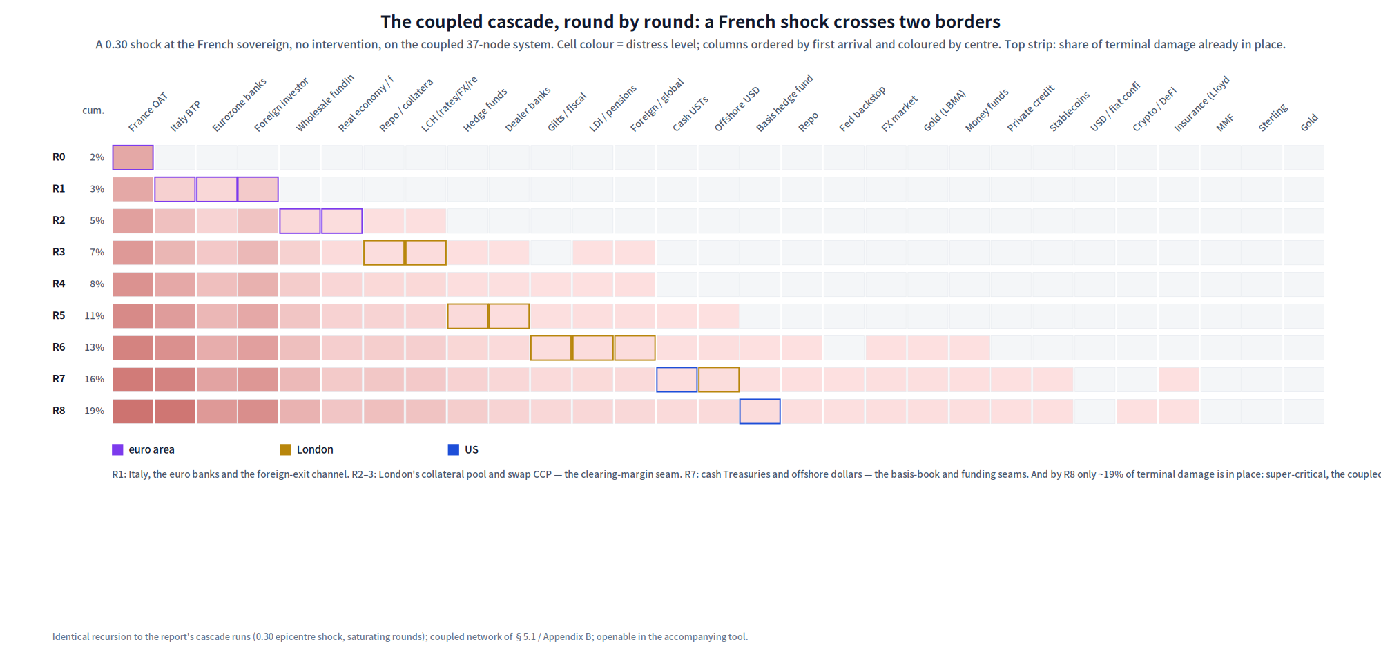
Figure 15 — The coupled cascade, round by round: a French shock crosses two borders. A 0.30 shock at the French sovereign on the coupled 37-node system, no intervention; columns ordered by first arrival and coloured by centre; outlined cells mark first arrival. Italy, the euro-area banks and the foreign-exit channel are hit in round 1; London’s collateral pool and swap clearing house by rounds 2–3 — the clearing-margin seam; cash Treasuries and offshore dollars by round 7 — the basis-book and funding seams. By round 8 only about a fifth of terminal damage is in place: the super-critical coupled run saturates the whole system, a slow burn with no internal stop.

§5.1’s reading rests on ten weights set by mechanism class, and the honest objection is that a coupled amplification factor is only as firm as those weights. Part 1’s dynamic method answers the objection without waiting for the full flow calibration. We hold the three block calibrations frozen and let the ten cross-centre edges breathe with an observable dollar-funding spread — three-month financial commercial paper minus the three-month Treasury bill, the standard gauge of dealer and money-fund dollar-funding stress — exactly as Part 1’s ρ(t) let a network’s binding edges re-sample from a live series while the topology stayed fixed. The result is a curve, not a point (Figure 16). As the funding spread compresses toward zero the cross-centre edges vanish and the amplification factor falls to the largest single block — 0.977, the US complex alone, subcritical. At the normal, median spread the mechanism weights reproduce 1.11. The threshold is crossed at a cross-centre spread of roughly four basis points: the coupled system is supercritical at essentially any normal funding state, and returns below the line only when the spread is compressed to near zero — that is, only when central-bank liquidity floods the cross-centre dollar-funding market completely. What holds the coupled structure below the threshold is therefore not the structure but the flood: continuous official liquidity keeping the funding seam compressed. The spread carries a policy-cycle component, so the curve is read for its shape and its critical region rather than for point values, and calibrating every edge in full from flow data remains beyond this report (§5.5 takes the available intermediate step: one observable per edge family, read monthly); but the reading no longer rests on a single static estimate, and the mechanism weights sit on the curve where a normal funding state puts them.

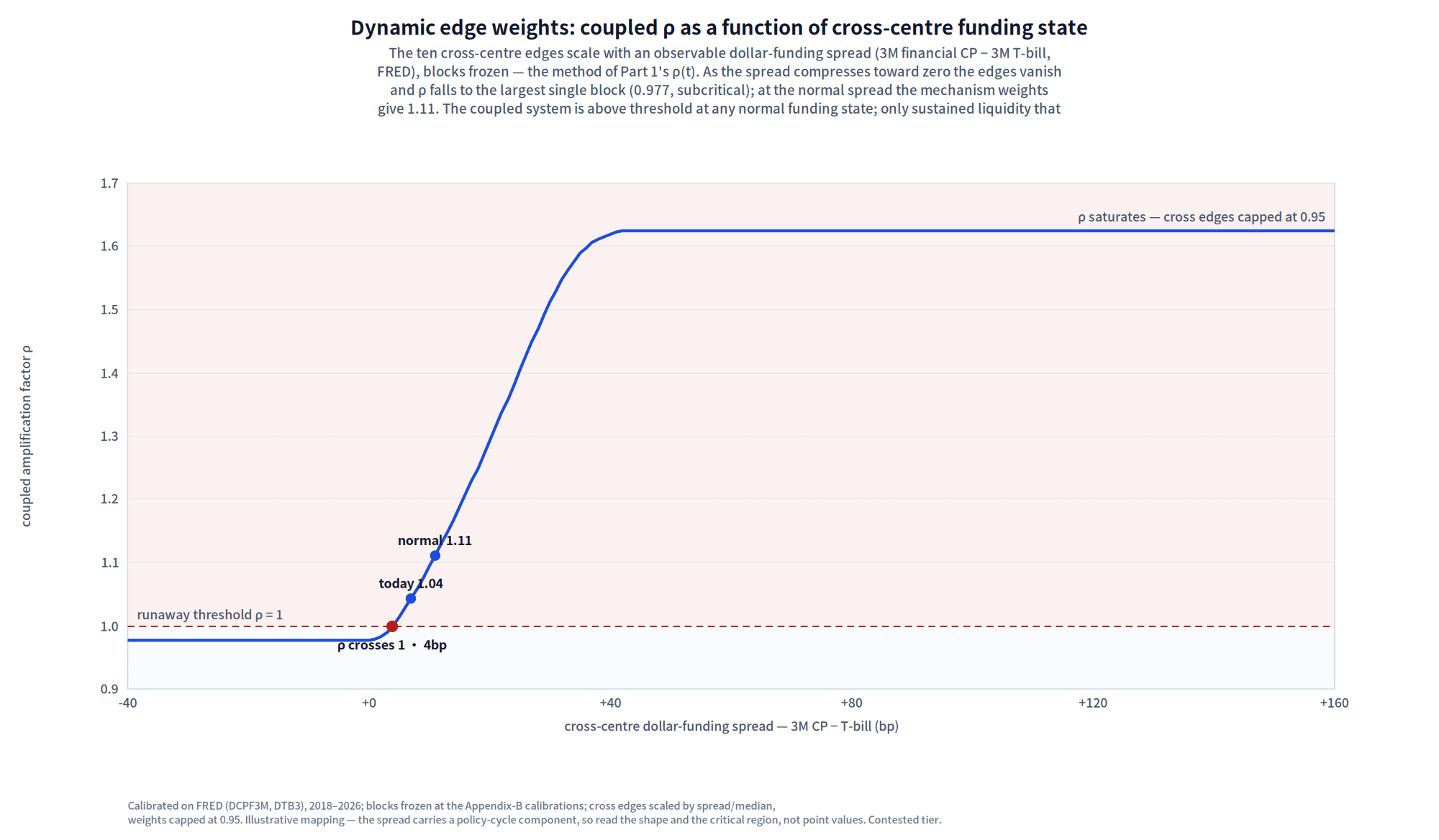
Figure 16 — Dynamic edge weights: coupled ρ as a function of cross-centre funding state. The ten cross-centre edges scale with an observable dollar-funding spread (three-month financial commercial paper minus the three-month Treasury bill, FRED), the three block calibrations frozen — the method of Part 1’s ρ(t). As the spread compresses toward zero the cross-centre edges vanish and ρ falls to the largest single block (0.977, subcritical); at the normal spread the mechanism weights give 1.11; the threshold is crossed at a cross-centre spread of about four basis points. The coupled system is above threshold at any normal funding state, and only sustained liquidity compressing the spread to near zero holds it under one. The spread carries a policy-cycle component, so the curve is read for shape and critical region, not point values. Contested tier; calibrated on FRED, blocks frozen at Appendix B.

5.2 The containment scorecard — and the gauge that reads no structure

Part 1 closed its structural readings with two further instruments, and the framework’s discipline requires both here. The first is the containment scorecard: three gates a rescue must pass — deployed (speed and will), sized and type-matched (the tool fits the loop geometry), affordable (the fiscal and monetary room to fund it) — scored as sourced judgement, pass = 1, partial = ½, fail = 0. Applied to London and the euro area, with Part 1’s reading of the United States carried over:

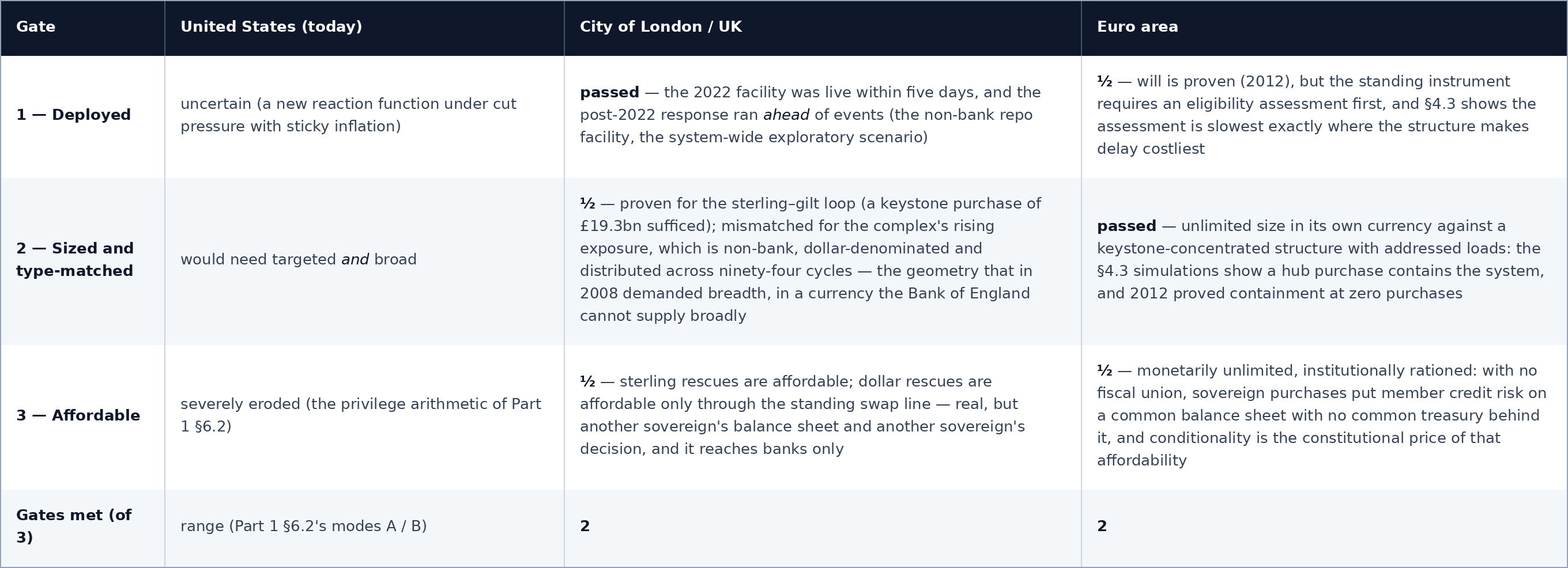
The scores are less informative than their decomposition. All three centres sit near two gates, but they miss different gates, and the miss in each case is the §5 table’s gap restated in containment vocabulary. The United States’ binding gate is arithmetic: the will and the tools exist, and what erodes is the affordability behind them — the privilege itself (Part 1, §6.2). London’s binding gates are geographic: the will is the best-proven of the three — 2022 is the record’s cleanest deployment, and the post-2022 reforms are its only pre-emptive containment — but the tools reach sterling and banks, while the exposure has migrated to dollars and non-banks; its affordability on the dollar side is borrowed. The euro area’s binding gates are constitutional: the currency is unlimited and the structure is the most single-point-rescuable of the three, but the speed of deployment and the unconditionality of funding are both rationed by the union’s own rules. Three centres, three different open doors: a common shock would enter each through a different failure.

Placed on Part 1’s structure-times-containment plane, the two European centres occupy instructive corners. London combines a 2008-shaped structure — feedback dispersed across ninety-four cycles, circulation 0.89, no single load above eleven per cent — with two gates met: the structure that would demand the broadest rescue is held by the centre whose broad-rescue currency is not its own. The euro area is the 1929 column inverted. In 1929 the structure was among the most rescuable on record and the rescuer was absent by doctrine; the euro area’s structure is likewise concentrated and addressable — and its rescuer is present but bound by its own constitution. 1929’s gate failed by belief; the euro area’s is conditioned by design. Whether that design opens in time is precisely the eligibility question of §4.3.

The second instrument is the drift gauge — the Fisher–Rao regime distance of Part 1 §3.4, which reads only a market series and shares no input with the calibrated networks. It had not yet been run for these centres; it now has, on daily ten-year series from the public sources the tool fetches directly: the nominal gilt curve (Bank of England), the euro-area all-bonds curve (European Central Bank), and the US Treasury benchmark, each from 2006, with the calm baseline chosen by the fixed rule, never by hand. The gauge dates the record’s crises without being told about them: the gilt series’ maximum distance falls on 21 October 2022 — the closing week of the liability-driven-investment crisis — and the US series’ abnormality companion peaks on 3 December 2007, the same early dating of the funding break that Part 1 reported. (One honest caveat: the euro-area aggregate nets core against periphery, so the 2010–12 divergence crisis is understated by construction; the series’ maximum falls instead in the first week of July 2022, the fragmentation scare that produced the Transmission Protection Instrument.) Today all three series read calm: the gilt at the 57th percentile of its own history, the euro-area curve at the 33rd, the US at the 16th, with the abnormality score negative in each case. That calm is the finding. The structural dials of this report read near-critical and, coupled, super-critical; the one instrument that reads no structure reports quiet — which is exactly the configuration the report has claimed throughout: taut wiring under quiet prices. The gauge cannot confirm the wiring; what it confirms is that the wiring readings are not echoes of current market stress — and on the one occasion in each centre’s recent record when the structure did fire, the gauge moved to its historical maximum within days.

On the framework itself, the three-centre exercise is a fair test of whether the lenses earn their keep, and the answer is that they disagree in the informative way. The amplification dial ranks the euro area tautest; the anatomy ranks London’s structure the more dangerous shape; the scorecard ranks their containment equal in score and opposite in kind; the drift gauge reads all three calm. No single lens carries the conclusion, and no two tell the same story — which is what a multi-lens framework is for. Where they converge — every centre one room internally, every exposure migrated to where its own backstop does not reach, the coupled system above the threshold each part sits below — the convergence is the finding.

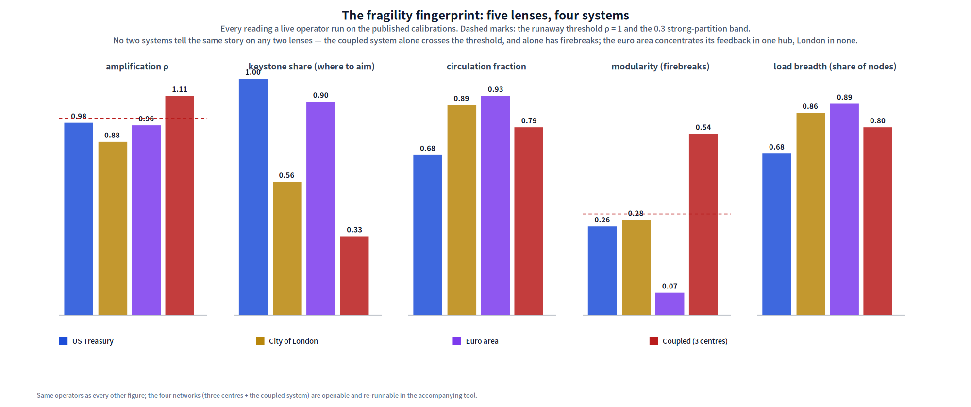
Figure 17 — The fragility fingerprint: five lenses, four systems. Amplification, keystone share (where a backstop can aim), circulation fraction, modularity, load breadth — every reading a live operator run on the published calibrations. The euro area concentrates its feedback in one hub and has the fewest exits; London concentrates nowhere and carries the broadest load; the United States loads the asset itself; and the coupled system alone crosses the runaway threshold — and alone shows firebreaks (modularity 0.54): the three centres themselves, with the ten cross-centre channels as the doors.

5.3 The width, speed, and asymmetry of transmission

A model reading that three coupled centres cross the runaway threshold is only as good as the channels it couples through. Two questions decide whether that reading matters: how wide are the ten channels — could they carry a systemic shock — and how fast do they transmit. Width decides whether a reading above the threshold is a policy problem or a curiosity — amplification along thin pipes matters little, along trillion-dollar trunks a great deal; speed decides what kind of backstop could ever catch it — a channel that transmits in days can only be met by a facility that already stands, and any rescue that requires an assessment, a vote or legislation is late by construction. The record has already priced both, and the answers are not reassuring (Figure 18).

The channels are not thin pipes; they are trillion-dollar trunks. The offshore-dollar seam is the widest: European banks’ US dollar claims fell by $1.5 trillion in the eighteen months to March 2009 as this channel seized, and the official replacement — the Federal Reserve’s swap-line network — peaked at $583 billion outstanding on 17 December 2008, more than a quarter of the Fed’s balance sheet, deployed to plug precisely the gap this edge represents (McGuire and von Peter 2009; Federal Reserve 2013). The money-fund seam is comparably wide: on the eve of the 2011 stress, United States prime money funds held roughly a quarter of their assets in euro-area bank paper, and when they withdrew, the ten largest cut their European exposure by 45 per cent; in the sharper 2008 episode, $350 billion was redeemed from prime funds in eleven business days, cutting off some $175 billion of funding to non-US banks (Investment Company Institute 2011; Kacperczyk and Schnabl 2013). The basis and clearing seams carry the trillion-dollar Treasury position and roughly four-fifths of euro swap clearing that §3.5 and §4.4 already documented. Every one of the ten edges the coupling rests on has, behind it, a stock large enough to transmit a systemic shock.

Speed is the second axis, and the record shows three regimes. The dollar-funding channels transmit in days: in 2008 the offshore-dollar market seized within a week of the Lehman failure, and the swap lines were scaled up over the following fortnight. The money-fund channel transmits in months: the 2011 withdrawal from euro-area banks — the “quiet run” — played out from May to December, the slow-burn shape the coupled cascade itself takes, where by round eight only a fifth of the damage is in place (§5.1). And a channel that is intercepted transmits nothing across borders: in 2022 the Bank of England’s keystone purchase arrested the gilt spiral within five days, and no measurable stress crossed to New York or the euro area — the containment counterfactual, run once by history.

Transmission is not symmetric, and three facts from the record fix its shape. First, the United States is the strongest and fastest transmitter, because dollar funding is universal — the finding of the global-financial-cycle literature (Rey 2013), of the cross-border banking data (McGuire and von Peter 2009), and of the directional-connectedness measures that rank the US a net volatility transmitter to Europe (Diebold and Yilmaz 2014). Second, Europe transmits to the United States through specific seams rather than broadly: the 2011 episode reached US money funds through the euro-bank paper they held, a channel-specific slow run, not a general shock. Third, London is rarely the origin and usually the amplifier — the role it played in 1931, when the Central European panic reached Britain not directly but through the London acceptance houses that had guaranteed German commercial bills, and the resulting liquidity strain contributed to sterling’s departure from gold that September (Accominotti 2012). That last case carries the anatomy finding of this report a century early: Accominotti’s central result is that organisation decided exposure — the large, diversified American commercial banks were barely touched by the Central European freeze, while the small, specialised London merchant banks were breached. It is §5.2’s scorecard in historical form: what breaks is not the most exposed centre but the one whose structure routes the shock through a node its backstop does not reach.

The width and the speed are not conjecture; they are magnitudes the historical record has already paid to contain — which is what makes §5.1’s coupled reading a policy problem rather than an artefact on paper.

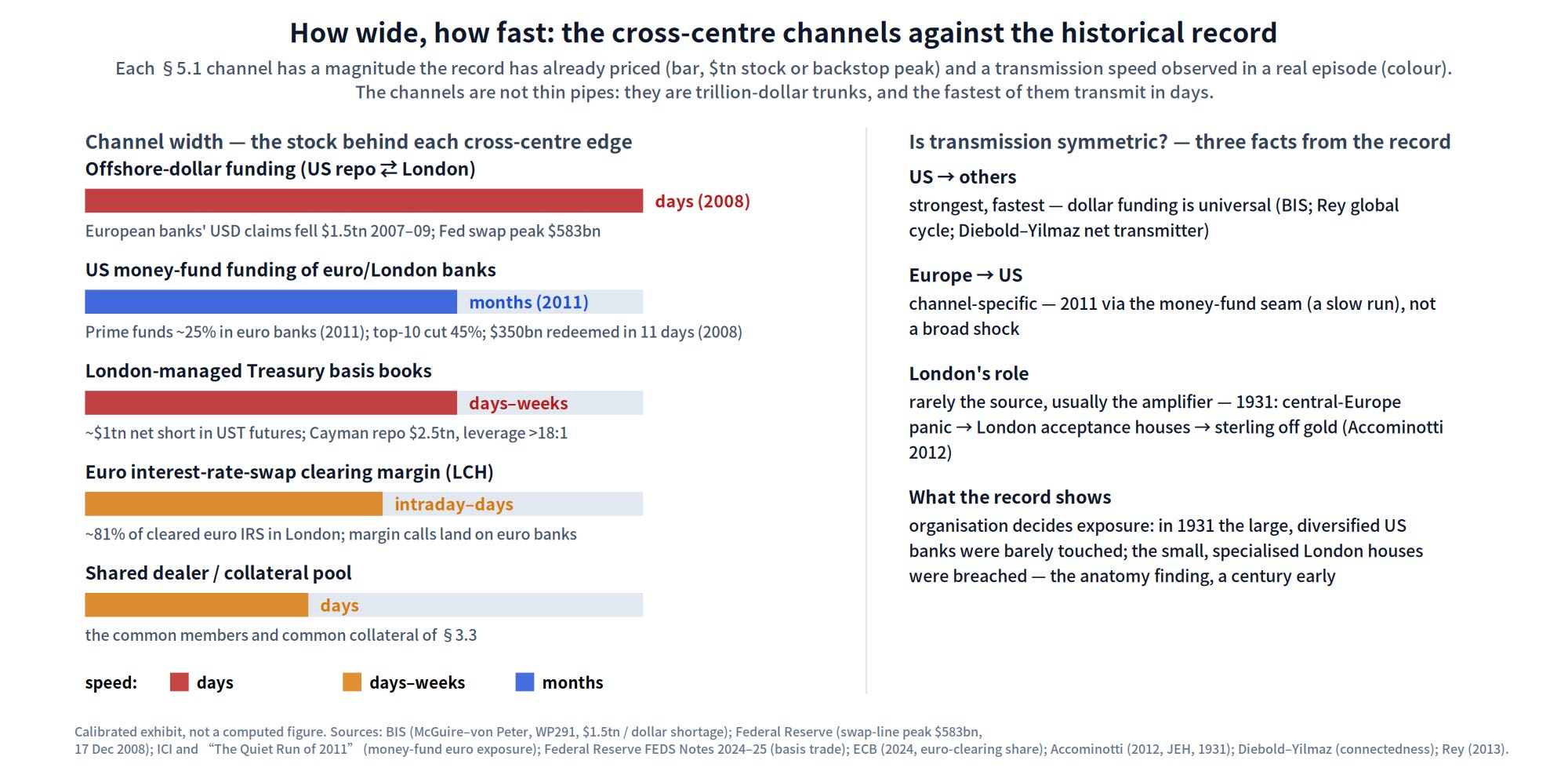
Figure 18 — How wide, how fast: the cross-centre channels against the historical record. Each of the ten §5.1 channels has a magnitude the record has already priced (bar length — the stock behind the edge, in $tn, or the official backstop peak) and a transmission speed observed in a real episode (colour: days / days–weeks / months). The offshore-dollar seam is the widest and among the fastest (2008, days; Fed swap peak $583bn); the money-fund seam is comparably wide but slow (2011, months). Right: three facts on the asymmetry of transmission from the record — the US as universal transmitter, Europe reaching the US through specific seams, and London as the historical amplifier (1931). A calibrated exhibit, not a computed figure; sources in the caption.

5.4 Three historical replays: the coupled system against the record

A calibrated network should be falsifiable against history, and the record offers three crossings to test: seed the network with an episode’s originating shock and check whether distress arrives where the record says, in the order the record says, at the tempo the record says. We replay 2008, 2011 and 1931 on the same frozen coupled network of §5.1 (Figure 19). Nothing is re-fitted per episode; only the seed changes.

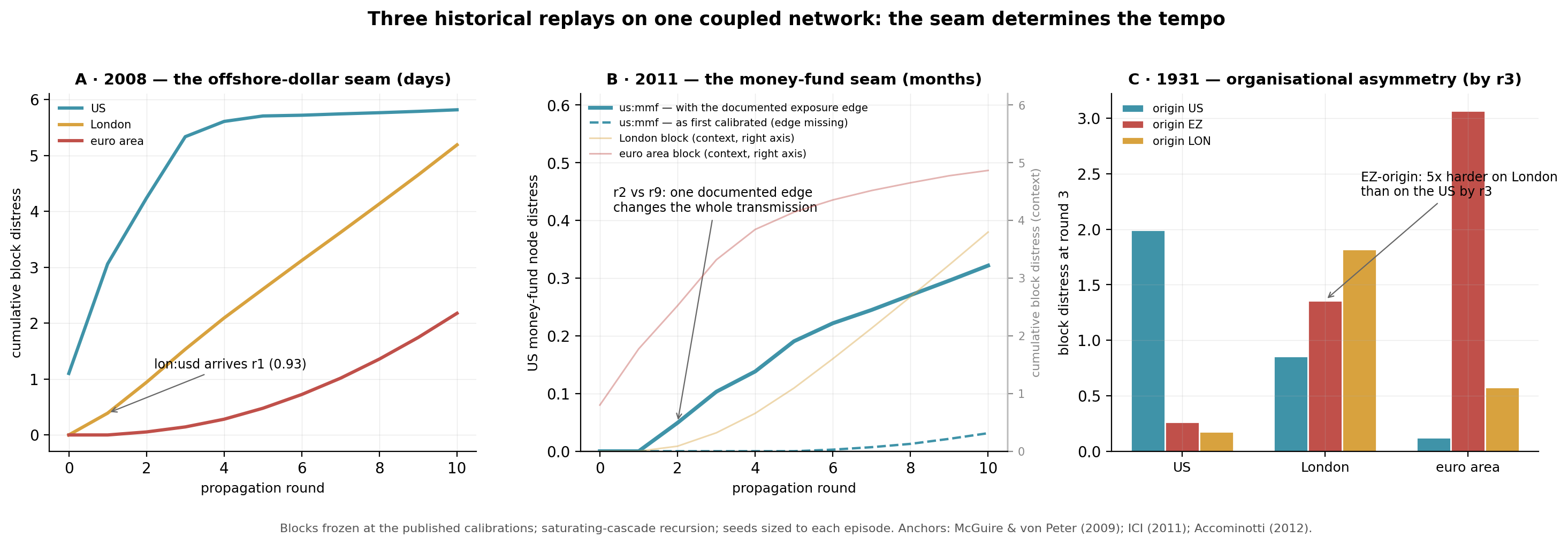
Figure 19 — Three historical replays on one coupled network: the seam determines the tempo. Panel A: a shock to the US funding core; the London offshore-dollar node is the first foreign arrival (round 1, 0.93), the recorded order and the fast tempo of 2008. Panel B: euro-sovereign stress; the US money-fund node (left axis) arrives at round 2 only on the amended network (solid) — on the first calibration, which carried the funding direction but not the exposure direction, it stays dark until round 9 (dashed); the origin blocks are drawn faint against the right-hand axis for context. Panel C: the same shock from each origin, damage by round 3 — the euro-origin shock lands about five times harder on London than on the US, Accominotti’s 1931 asymmetry reproduced structurally.

2008, the offshore-dollar seam — order and tempo reproduced. Seeding the US funding core, the London offshore-dollar node is the first foreign arrival, in round 1 and almost saturated (0.93); London collateral and repo follow in round 2, euro wholesale in rounds 2–3. That is the recorded order — the offshore dollar market froze within days of Lehman, before continental balance sheets showed strain — and the recorded tempo: 35 per cent of terminal system damage lands by round 3, the fast profile. The widths of Figure 18 give the scale the replay stands on: the $1.5 trillion contraction in European banks’ dollar claims, met by the $583 billion swap-line peak.

2011, the money-fund seam — the quiet run, and a missing direction found. This replay produced the one amendment this section makes to §5.1’s network, and we report it as method rather than bury it as a fix. As first calibrated, the coupled network could not reproduce the episode at all: the euro-sovereign shock reached the US money-fund node only at round 9, as a faint echo. The reason was directional. The mechanism calibration had encoded the funding direction — US money funds lend to European banks — but not the exposure direction: when European banks are distressed, it is the funds holding their paper that mark the damage. That second direction is thoroughly documented — prime funds held roughly 30 per cent of assets in euro-area bank paper in May 2011, and the largest funds cut that exposure by about 45 per cent over the following seven months (Kacperczyk and Schnabl 2013; Chernenko and Sunderam 2014) — so the edge enters the network with its source, as an eleventh channel. With it, the money funds light up at round 2, and the tempo is the opposite of 2008: 17 per cent of terminal damage by round 3, 42 per cent by round 8 — the slow burn of an episode that ran from May to December without a single crisis day. The amendment moves the coupled reading from 1.11 to 1.12 and strengthens, rather than disturbs, every robustness statement of §5.1 (each was computed on the sparser ten-channel network). The lesson stands on its own: direction is calibration, and a missing direction is invisible until an episode demands it — one documented edge changed an episode’s entire transmission, which states the case for the flow-data programme better than any argument.

1931, the organisational asymmetry. Accominotti’s finding — the central-European panic broke London’s specialised acceptance houses while America’s diversified banks were barely touched (§5.3) — is a claim about where early damage lands, and on a supercritical network it must be read in the early rounds, because terminal damage converges wherever the shock starts. It is there (Figure 19, panel C): a euro-origin shock lands roughly five times harder on London than on the US by round 3 (1.36 against 0.26), and reaches London’s banks two rounds before it reaches US funding. A US-origin shock reaches London fastest of all (round 2, through the offshore-dollar seam); a London-origin shock reaches both other centres by rounds 1–2 — the amplifier’s role, §5.3’s third asymmetry fact. A twentieth-century organisational fact survives into a twenty-first-century calibration because it lives in the topology, not in the era.

Across the three replays the cross-cutting result is the one a single number cannot show. The static coupled reading says whether the system amplifies; the replays say where the damage lands and how fast — and both answers depend on which seam the shock enters through, not on the size of the shock. The same graph transmits in days through the offshore-dollar seam and in months through the money-fund seam. For surveillance this is not a nuance: a monitoring framework calibrated to one tempo will be early or late at the other, and which tempo applies is a property of the seam.

5.5 How tight is it now: the coupled reading as a monthly series

FFigure 16 made the coupled reading a curve over funding states; this section makes it a series over time, one step short of the full flow calibration. First, what the instrument is for. It is the closest this construction comes to a backtest: had the gauge been running since 2019, it should light up in the right months, for the right reasons — the record below checks exactly that. And it separates the two states a policymaker most needs to tell apart: pressure months, when funding prices light up and the system is under stress now, and tight months, when positioning stacks to record percentiles while every price stays quiet — the system fuelled, not yet ignited; the two call for entirely different responses, and on any single price gauge the second is precisely the one that stays invisible. Each cross-centre edge is driven by the observable that most plausibly gates it, in two families read differently — a distinction we learned by getting it wrong. Price wedges — the commercial-paper–bill spread for the dollar term-funding edges, overnight-rate-to-policy-floor wedges for sterling and euro conditions — are read as deviations from their own trailing history (a causal score, no look-ahead). Positioning and level series — the CFTC leveraged-fund net short across Treasury futures for the basis edges, realized volatility of the twenty-year gilt yield as a margin-pressure proxy for the clearing and collateral edges — are read as expanding percentiles of their level, because a positioning stock near its record can read as normal against a trailing median that the build-up itself has dragged up. Levels measure vulnerability; deviations measure momentum; confusing them mutes exactly the episodes one most wants to see. Two further lessons are built in: fast policy cycles move the paper–bill spread through the instruments’ maturity mismatch rather than through dealer constraint, so the dollar term leg is capped in quarters where the policy rate moves forty basis points or more; and month-end sampling misses intra-month spikes — the March 2020 stress peaked mid-month and was half-erased by facilities before the 31st — so each month is read twice, at its median (the creep view) and at its within-month maximum (the spike view). Figure 20 plots both.

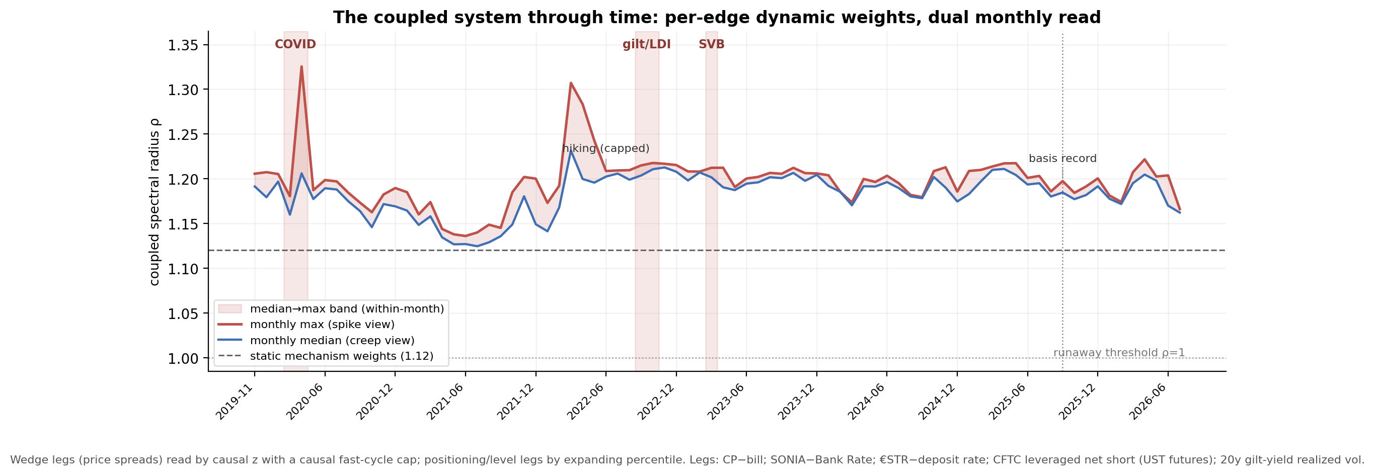
Figure 20 — The coupled system through time: per-edge dynamic weights, dual monthly read.

The series behaves as the record demands, which is the point of building it. March 2020 is the tightest month in the window (maximum ≈ 1.33), carried simultaneously by the sterling overnight wedge, the basis book and gilt volatility. The 2022 hiking months — which a naïve wedge reading would crown — are muted by the cap. The gilt months of September–October 2022 are lit by the collateral-volatility leg at its 100th percentile, an event to which every overnight-rate gauge in the set is blind: precisely why the clearing edges need a margin-sensitive leg. March 2023 and the September 2025 record in basis positioning are visible at the right times. And the present: mid-2026 reads about 1.17 against the static 1.12, with the tension carried not by the funding wedges — all quiet — but by a Treasury-basis position at its 86th percentile in aggregate and its 91st percentile in the ten-year contract alone, the same series whose 2020 unwind Part 1 documented. The system is not in a stress month; it is in a tight-positioning month, and the gauge exists to tell those apart: quiet funding over record positioning is the configuration this report has called taut wiring under quiet prices, now stated as a number with a decomposition rather than a phrase.

6. Conclusion: what the no-privilege cases add, and what to watch

Part 1 found a near-critical US structure held by privilege. Part 2 finds that privilege is not a single thing one either has or lacks, but a set of reaches — over a currency, over counterparties, over a sovereign’s debt — and that the centres without the full set are not uniformly more fragile, but differently exposed. The City of London produces liquidity in currencies it cannot issue and runs near-critical on the structure that does it, with a backstop gap at the non-bank dollar and the shared clearing collateral. The euro area can issue the currency it runs on without limit yet has the most constrained backstop of the three, because a monetary union without a fiscal union cannot catch its members unconditionally, and the conditionality binds hardest where the fragility is now migrating.

Three things to watch follow directly, and each is a live, measurable indicator rather than a forecast:

1. Non-bank dollar leverage in and through London. The basis trade and gilt-repo leverage are at records and concentrated in a handful of funds; the indicators to track are the net futures positions, the repo borrowing, and the leverage ratios the official sector already publishes — and whether a non-bank, dollar facility is built before they are tested (Financial Stability Board 2025; Bank of England 2025b).

2. France and the conditionality assessment. Whether France’s adjustment keeps it eligible for the euro-area backstop, and whether the European Central Bank pre-clarifies how it would treat a systemically-core member whose stress is political rather than purely fundamental, decides whether the tool can fire where it would now be most needed.

3. The clearing that has not moved. The euro area’s inability to move the clearing of its own currency out of London is a standing measure of how bound the two centres are; the share of euro clearing in London is the simplest single gauge of a dependency that no amount of strategic-autonomy policy has shifted.

This report is the second in a series. It treats the City of London at the depth its position warrants and reads the euro area as the counterpoint that sharpens the comparison. We note only that the method that locates a gap in London’s clearing collateral is the same method that would locate the analogous gap elsewhere, and that the value of the series, if it has one, is not in any single map but in the fact that every map in it can be opened, re-run and checked.

An earlier report (Gao 2026b) argued that the world’s critical dependencies have become chokepoints — single points through which a shock to one party is a shock to all — and traced one such stack through the physical, geopolitical and financial layers of the global AI build-out. The City of London is, on the reading here, a financial chokepoint of the same kind: the place where the world’s foreign exchange, its euro clearing and its offshore dollars are priced and transferred, bound together by a collateral pool that a central bank issuing the wrong currency cannot fully reach. The two readings meet at a specific concern: that report identifies the debt-funded expansion of the AI complex as a rising source of pressure on sovereign credit, and the present one measures how a shock to sovereign credit would propagate through centres that cannot, by construction, fully backstop it. How a shock at one centre becomes a shock at the others is measured in §5.1’s coupled reading — three subcritical centres joined by their documented channels read above the runaway threshold — and tested against the record in §5.4; the periphery those centres drive, from Asia to Latin America, lies beyond this report’s scope. That is not a cause for alarm. It is a reason to know precisely where the gap is — which is what this report has tried to establish.

Appendix A — Method and simulation definitions

The lenses are defined formally in Part 1 (Gao，2026a), Appendix A, and are not re-derived here; the same code computes every reading in both reports. In summary: a financial complex is a directed weighted graph in which the weight on edge i → j is the fraction of a unit distress shock at balance sheet i that is transmitted to j.

The amplification factor ρ is the spectral radius (largest absolute eigenvalue) of that weighted adjacency matrix; for ρ < 1 the steady-state multiplier of a shock is 1/(1−ρ), and ρ = 1 is the runaway threshold (May 1972).

The loop-concentration reading is a Herfindahl-type index over the gains of the network’s feedback cycles (low = distributed, high = one dominant loop); the keystone is the node carrying the largest share of cycle gain.

The cascade is a saturating reverberating propagation (the DebtRank family; Battiston et al. 2012) from a seeded shock, reporting the per-node distress at convergence.

The backstop simulation extends the cascade with a standing purchase facility at a designated keystone node k: from an activation round t₀ the facility absorbs a fraction a of the distress flow arriving at k each round, before it materialises as damage. The facility cannot pre-absorb the initial shock and cannot stop the keystone’s own first-wave transmission; t₀ = ∞ or a = 0 reproduces the unrescued cascade exactly. Figures 5, 10 and the intervention readings in §3.5 and §4.3 use a 0.30 epicentre shock, a = 0.9 and t₀ = round 2; the timing-and-size discussion in §4.3 sweeps t₀ and a. The early-intervention leverage quoted throughout, and plotted in Figure 13, is 1/(1−ρ), evaluated at each centre’s amplification factor.

The sensitivity analysis of §2.3 and Figure 1 perturbs every calibrated edge weight of a network by an independent uniform factor 1 + u, u ∈ [−p, +p] for p ∈ {0.15, 0.20, 0.30}, clips the result to [0, 1], and recomputes ρ and the keystone for each of 2,000 draws per level, under a fixed pseudo-random seed. Reported are the 5th, 50th and 95th percentiles and the full range of ρ, and the share of draws in which each node is the keystone. Every figure is reproducible by opening the named, calibrated network and re-running these operators.

Appendix B — Calibrations and figure data

The City of London network is eighteen nodes and forty-four weighted edges. Its edge weights are set by mechanism class — margin and clearing pass-through 0.40–0.45, funding withdrawal 0.35–0.40, reflexive asset-sale 0.28–0.35, collateral and haircut 0.28–0.32, contagion and spillover 0.20–0.30, inflation and currency 0.20–0.25 — and are not tuned to a target amplification factor; the operators return ρ = 0.881, keystone the interest-rate-swap clearing house (cycle-gain share 0.564), loop concentration 0.095 (distributed), 94 cycles, effective load breadth 15.4 of 18. The anatomy (§3.2): top engines LCH⇄repo 0.16 and dealer banks⇄offshore dollars 0.14, then hedge funds⇄repo 0.10 and gilts⇄LDI 0.08; self-reinforcing core 13 of 18 (the commodity clearing houses and the central bank on one-way roads into it); heaviest single load ≈ 11 per cent (repo-collateral), load concentration 0.074; circulation fraction 0.889; modularity 0.281 (below the 0.3 firebreak band). Under a ±20-per-cent perturbation of every edge (§2.3) ρ stays within roughly 0.84–0.92 and the keystone stays on the clearing-and-collateral complex in every draw. The load-bearing clearing-and-collateral loop is calibrated to the 2022 liability-driven-investment episode — collateral and margin calls in excess of £70 billion on a roughly 130-basis-point gilt move (Bank of England 2022) — and is, on that anchor, conservative, since the interest-rate clearing house clears a multiple of the gilt market alone. The full node-and-edge table, with the mechanism and source for every edge and a calibrated/estimated label, is in the working calibration document and is reproduced in the openable network.

The UK liability-driven-investment network (2022) is eight nodes; the operators return ρ = 0.914 (range ≈ 0.83–0.99 at ±20 per cent), keystone the leveraged hedging fund (cycle-gain share 1.0), one dominant loop. The reformed UK gilt network (today) is seven nodes and returns ρ = 0.609, keystone the gilt market, reflecting the raised resilience buffers; the fall from 0.914 to 0.609 is the structural signature of the 2022–23 reform, and the corresponding early-intervention leverage falls from 11.7 to 2.6 (Figure 13).

The euro-area networks carry over from Part 1’s European material: the 2010–12 sovereign-bank calibration (ρ = 0.971, range ≈ 0.91–1.03 at ±20 per cent, single peripheral-sovereign hub) and the today calibration (ρ = 0.963, keystone Italy with cycle-gain share 0.90, France carrying roughly a tenth of the feedback outside the hub), with two edges cross-validated against the 2012 episode and the remainder estimated by mechanism. The anatomy (§4.2): top engines Italy⇄foreign investors 0.23, banks–Italy–wholesale 0.12, banks⇄Italy 0.10, France⇄Italy 0.075; self-reinforcing core 6 of 7 (all but the quantitative-tightening node, which injects one-way); loads Italy 0.28 / France 0.18 / banks 0.17, effective breadth 6.3 of 7; circulation fraction 0.927; modularity 0.066 — the lowest in the series. Both are openable and re-runnable in the accompanying tool.

The coupled three-centre system (§5.1, Figure 14) joins the three published calibrations above — unchanged — with ten cross-centre edges, one per documented channel: offshore-dollar funding (US repo ⇄ London offshore-dollar, 0.40/0.30), the London-managed basis books (cash Treasuries ⇄ London hedge funds, 0.30/0.32), euro-swap clearing margin (London swap CCP ⇄ euro-area banks, 0.35/0.28), US money-fund wholesale funding of London dealer banks and euro wholesale (0.30 each), euro banks in the London collateral pool (0.25) and the dealer counterparty channel (0.25). Each weight is set by mechanism class within the same ranges as the block calibrations and is not tuned; the Fed–BoE swap line is a stabiliser, not a distress channel, and is therefore excluded from the edges and discussed as a backstop. The operators return: coupled amplification factor 1.112 against single-block readings of 0.977 / 0.881 / 0.963; conservative low-end coupling 1.066; ±20 and ±30 per cent Monte Carlo on the cross edges alone (blocks frozen, 500 draws per level, seed 20260702) keeps every draw above 1 (±30%: 5th–95th percentile 1.091–1.133); the threshold is crossed at roughly 0.5× the estimated coupling. Referee checks: leave-one-channel-out ρ ∈ [1.074, 1.109] (all ten drops above 1); leave-two-out over all 45 pairs ρ ∈ [1.019, 1.106], 100 per cent above 1; a random-rewiring null (the ten weights kept, endpoints redrawn across blocks, 500 draws, seed 20260703) crosses 1 in 63 per cent of draws with median 1.009 — generic destabilisation — while the documented wiring’s 1.112 sits above the null’s 95th percentile (1.062). An eleventh channel — the 2011 exposure direction, US prime funds’ holdings of euro-area bank paper (§5.4) — enters the replay and the dynamic series of §5.5; the static robustness suite above is computed on the ten-channel network and is strengthened, not weakened, by its addition (coupled reading 1.12). Coupled keystone: cash Treasuries at a cycle-gain share of 0.33 (single blocks: 1.00 / 0.56 / 0.90), loop concentration distributed, 371 cycles. The remaining lenses on the coupled system: circulation fraction 0.794 (blocks alone 0.677 / 0.889 / 0.927); community modularity 0.537 under a fixed-seed weighted partition, with the three communities exactly the three centres (every Part 1 crisis-eve network reads below 0.3); one self-reinforcing core of 27 of 37 nodes spanning all three centres; load entropy 0.94 (normalised), effective breadth ≈ 29 balance sheets, concentration index 0.041 — dispersed on the load axis as well as the feedback axis.

The euro-area centres map (Figure 11) is not a calibrated network but a data exhibit: eight financial centres positioned at their coordinates, sized by their Global Financial Centres Index 39 rating (London 766, Zurich 738, Frankfurt 734, Luxembourg 733, Geneva 731, Paris 730, Amsterdam 729, Dublin 722, Madrid 709, Milan 704), coloured by post-Brexit specialisation, over a country tint set by the sign of each member’s end-May-2026 TARGET balance (Germany +€1,066bn, Luxembourg +€205bn, and the debtor set led by Spain −€449bn, Italy −€359bn and France −€190bn). The binding lines are the shared depositories and clearing houses. The map’s constants live in one module that the figure script, the data endpoint and the tool’s euro-area lens all read, so the exhibit, the panel and the reproduction cannot drift apart.

Every figure’s underlying readings are computed live from these calibrated networks; the figure-generating script and the per-figure numbers are in the repository, and each network opens and re-runs in the accompanying tool.

Appendix C — Data feeds and reproducibility

Every reading rests on public series and documents, accessed June and July 2026 unless noted:

• Market structure — BIS Triennial Central Bank Survey 2022 (UK shares of global foreign-exchange and over-the-counter interest-rate-derivatives turnover, via the Bank of England); LSEG / LCH and the European Central Bank (euro interest-rate-swap clearing share, roughly 81 per cent in London as of December 2023); London Metal Exchange and LME Clear (metals clearing, the 2022 nickel event); London Bullion Market Association (gold vaulting); Lloyd’s and the International Group of P&I Clubs (insurance and global tanker liability cover); New Financial, Brexit & the City (post-Brexit relocation by city and asset class).

• Backstop toolkit — Bank of England gilt-market-operations statements (2022, the £19.3 billion purchase against a £65 billion ceiling); the Contingent Non-Bank Financial Institution Repo Facility explanatory note (2024); the gilt-repo-resilience discussion paper and the central-counterparty-resilience consultation and stress test (2024–25); Federal Reserve standing-swap-line and foreign-authority-repo announcements (2013, 2020) and the Treasury basis-trade FEDS notes (2024, 2025); FSB Leverage in Non-Bank Financial Intermediation (2025).

• Euro area — ECB statements on Outright Monetary Transactions (2012), the Transmission Protection Instrument (2022), the post-Brexit clearing landscape (2024) and capital-markets integration (2025); the Council of the EU excessive-deficit recommendation to France (2025); Insee (the 2025 French deficit and debt, released March 2026) and IMF (the 2025 France Article IV and Euro-Area Financial System Stability Assessment). The euro-area centres map (Figure 11) draws on the Global Financial Centres Index 39 (Z/Yen, March 2026) for centre ratings and on the ECB Data Portal’s TARGET-balance series (end-May 2026, cross-checked against the Deutsche Bundesbank’s published €1,065.7bn claim) for the liquidity axis.

• Time-series readings — no daily public series of clearing-house collateral or cross-border repo is available on a free official feed, so no time-path of the amplification factor is computed for these centres (stated, not hidden); the long-rate context uses monthly OECD series via FRED, identified in the calibration documents.

• Drift-gauge series (§5.2) — daily ten-year yields, fetched directly by the tool: the UK nominal zero-coupon gilt curve (Bank of England Interactive Database, series IUDMNZC), the euro-area all-central-government-bonds curve (ECB Data Portal, yield-curve dataset, 10-year spot), and the US constant-maturity benchmark (FRED, DGS10); window 2006 to present, calm baseline selected by the fixed objective rule of Part 1, Appendix A.5. Each run is re-executable in the accompanying tool from the same sources.

The figure-generating script, the calibrated networks, and the operator outputs are in the repository; each network is openable and re-runnable in the accompanying tool. The robustness suite (Figure 1 and the §5.1 checks: perturbation quantiles, keystone stability, leave-two-out, the null rewiring) and the dynamic-tightness readings (the Figure-16 curve, the Figure-20 monthly dual read, and the current-month decomposition) run as operators on the wired networks themselves, shipped pre-wired on the centre and coupled templates in the accompanying tool.

References

Accominotti, O. (2012) ‘London merchant banks, the central European panic, and the sterling crisis of 1931’, Journal of Economic History, 72(1), pp. 1–43.

Agence France Trésor (2026) Monthly bulletin, April 2026 (holding structure of negotiable government debt). Paris: AFT.

Al Jazeera (2026) France adopts 2026 budget after two no-confidence votes fail. Doha: Al Jazeera.

Bank of England (2022) Statement on the Bank’s gilt market operations. London: Bank of England.

Bank of England (2022b) BIS Triennial Survey of Foreign Exchange and Over-the-Counter Interest Rate Derivatives Markets — UK data. London: Bank of England.

Bank of England (2023) Financial Policy Committee: steady-state resilience for LDI. London: Bank of England.

Bank of England (2024) Contingent Non-Bank Financial Institution Repo Facility (CNRF) — explanatory note. London: Bank of England.

Bank of England (2024b) Ensuring the resilience of central counterparties — supervisory stress test results. London: Bank of England.

Bank of England (2025) Transitioning to a repo-led operating framework; collateral eligibility in the Sterling Monetary Framework. London: Bank of England.

Bank of England (2025b) Enhancing the resilience of the gilt repo market — discussion paper. London: Bank of England.

Bank of England (2025c) Ensuring the resilience of CCPs — consultation paper. London: Bank of England.

Bank of England (2026) The system-wide exploratory scenario: final report; and Enhancing the resilience of the gilt repo market — feedback statement. London: Bank of England.

Battiston, S., Puliga, M., Kaushik, R., Tasca, P. and Caldarelli, G. (2012) ‘DebtRank: too central to fail? Financial networks, the FED and systemic risk’, Scientific Reports, 2, 541.

Chernenko, S. and Sunderam, A. (2014) ‘Frictions in shadow banking: evidence from the lending behavior of money market mutual funds’, The Review of Financial Studies, 27(6), pp. 1717–1750.

Council of the European Union (2025) Excessive deficit procedure: recommendation to France. Brussels: Council of the EU.

Diebold, F. X. and Yilmaz, K. (2014) ‘On the network topology of variance decompositions: measuring the connectedness of financial firms’, Journal of Econometrics, 182(1), pp. 119–134.

European Central Bank (2012) Technical features of Outright Monetary Transactions. Frankfurt: ECB.

European Central Bank (2022) The Transmission Protection Instrument. Frankfurt: ECB.

European Central Bank (2024) The derivatives clearing landscape in the euro area three years after Brexit. Frankfurt: ECB.

European Central Bank (2024b) Economic Bulletin: the Eurosystem balance sheet and quantitative tightening. Frankfurt: ECB.

European Central Bank (2025) Advancing the capital markets union: harmonising securities post-trading. Frankfurt: ECB.

European Central Bank (2025b) Financial Stability Review, November 2025 (box: US dollar activities of European banks). Frankfurt: ECB.

European Central Bank (2026) TARGET balances of participating national central banks (ECB Data Portal, end-May 2026). Frankfurt: ECB.

Federal Reserve (2013) Standing U.S. dollar liquidity swap arrangements. Washington, DC: Board of Governors.

Federal Reserve (2020) Establishment of a temporary FIMA Repo Facility. Washington, DC: Board of Governors.

Federal Reserve (2020b) Central clearing and systemic liquidity risk. Finance and Economics Discussion Series. Washington, DC: Board of Governors.

Federal Reserve (2024) Quantifying Treasury cash-futures basis trades. FEDS Notes. Washington, DC: Board of Governors.

Federal Reserve (2025) The cross-border trail of the Treasury basis trade. FEDS Notes. Washington, DC: Board of Governors.

Financial Stability Board (2025) Leverage in non-bank financial intermediation — final report. Basel: FSB.

Full Fact (2022) The Bank of England hasn’t already spent £65 billion following the mini-budget. London: Full Fact.

Gao, Y. (2026a) The Geometry of Market Fragility, Part 1: .How Close Is the US Treasury Market to a Self-Amplifying Break? Preprint.

Gao, Y. (2026b) AI’s Chokepoints: the physical constraints, geopolitical playbooks, and financial fragility of the global AI build-out. SSRN Working Paper 6884598. Available at: https://ssrn.com/abstract=6884598.

IMF (2025) France: 2025 Article IV consultation; Euro Area: Financial System Stability Assessment. Washington, DC: International Monetary Fund.

Insee (2026) In 2025, the public deficit stands at 5.1% of GDP, the public debt at 115.6%. Paris: Insee.

International Group of P&I Clubs (2024) Annual review: protection and indemnity cover and the world tanker fleet. London: International Group of P&I Clubs.

Investment Company Institute (2011) Money market funds and the eurozone: prudent response to European challenges. Washington, DC: ICI.

Ivashina, V., Scharfstein, D. S. and Stein, J. C. (2015) ‘Dollar funding and the lending behavior of global banks’, Quarterly Journal of Economics, 130(3), pp. 1241–1281.

Kacperczyk, M. and Schnabl, P. (2013) ‘How safe are money market funds?’, Quarterly Journal of Economics, 128(3), pp. 1073–1122.

London Bullion Market Association (2024) The global OTC bullion market. London: LBMA.

London Metal Exchange (2024) Clearing. London: LME.

London School of Economics (2025) How the EU is repatriating clearing services in the pursuit of financial autonomy. EUROPP blog. London: LSE.

May, R. M. (1972) ‘Will a large complex system be stable?’, Nature, 238, pp. 413–414.

McGuire, P. and von Peter, G. (2009) The US dollar shortage in global banking and the international policy response. BIS Working Papers No. 291. Basel: Bank for International Settlements.

New Financial (2021) Brexit & the City: the impact so far. London: New Financial.

The Pensions Regulator (2024) Improved resilience of LDI funds. Brighton: TPR.

Rey, H. (2013) ‘Dilemma not trilemma: the global financial cycle and monetary policy independence’, in Proceedings of the Federal Reserve Bank of Kansas City Economic Symposium, Jackson Hole.

Scope Ratings (2025) Italy: domestic investors vital for supporting government funding as market conditions shift. Berlin: Scope Ratings.

World Federation of Exchanges (2021) Procyclicality of CCP margin models: systemic problems need systemic approaches. London: WFE.

Z/Yen (2026) The Global Financial Centres Index 39. London: Z/Yen Group

Disclaimer. All exhibits and calculations in this report are computed directly on the Pangura Axe platform, drawing on publicly available market data. Pangura provides analytical infrastructure for decision-making by financial institutions and does not provide investment advice.